Tutorials Data Himalaya
The tutorial is prepared to use the J2000 hydrological model for hydrological system analysis of a river catchment. A test catchment and dataset of the Dudh Kosi river basin has been provided along with the tutorial. The Dudh Kosi river basin was used for the hydrological system analysis by using the J2000 hydrological model as a part of the PhD research (Nepal, 2012). The information provided here is largely based on this study. PhD Thesis. The motivation, objectives and methodological apporach and the rational of using the J2000 model in the Dudh Kosi river basin are also presented. The users can use the test data to get familiar with the model application. At the same time, users can prepare their own dataset to understand the hydrological system dynamics of any river basin by following this tutorial.
Contents |
Who can use the tutorial
The tutorial is prepared in such a way that the J2000 hydrological model can be used independently without any techtical support from model developers. Therefore, it can be used by students, model developers and researchers for the hydrological system analysis of a catchment. The tutorial should be read in conjunction with other sub-tutorials which has been mentioned in different part of this tutorial. Additionally, the tutorial is supplied with test dataset of the Dudh Kosi river basin (Nepal, 2012) which users can use to get familiar with the different aspects of the J2000 model. Similarly, users can also create their own dataset of the catchment of interest to run the model.
Description of the test dataset
The tutorial is accompained by the test dataset of the Dudh Kosi river basin. This hydro-meteorological data were provided by the Department of Hydrology and Meteorology (DHM), Government of Nepal. The DHM has provided permission to use the data along with the tutorial. The users are expected to use the tutorial along with the test data to understand different aspects of the J2000 modelling system and also aim to prepare their own dataset to run the model.
Motivation
This is the motivation of the study.
Study area
This is the Study area, Dudh Kosi river basin.
Objectives and methods
The main objectives of the
Preparation of dataset
Model parameter files
The requirement of the data to run the J2000 hydrological model is discussed in detail which is a pre-requisite to run the model. Two types of data are required i) model parameter files and ii) meteorological input data. The first one is prepared and quantified inside the GIS environment and known as model parameter files. The parameter files and their values are static in the modelling application.
Users have to prepare all the input data (i.e. soil, land cover, geology, DEM) in raster format with certain resolution. While delineating HRUs, all the input data has to be provided in a same resolution. The resolution of the dataset mainly controls the number of HRUs to be formed without loosing the heterogeneity of a catchment. Therefore, the resolution of input data depends upon a catchment to be modelled. If the catchment is small (e.g. 600 km²), the resolution between 30-90 is suitable depending upon the resolution of the available dataset. Similarly, for meso-scale catchment (e.g. 4000 km²), resolution between 250-500 m is suitable.
The detailed descriptions to derive the parameter files are provided below:
Soil parameter file
The detailed information required for the soil parameter file is provided in Table below.
| Parameter | Description |
|---|---|
| SID | soil type ID |
| depth | depth of soil |
| kf_min | minimum permeability coefficient |
| depth_min | depth of the horizon above the horizon with the smallest permeability coefficient |
| kf_max | maximum permeability coefficient |
| cap_rise | Boolean variable, that allows (1) or restricts (0) capillary ascension |
| aircap | air capacity (equivalent to large pore storages (LPS)) |
| fc_sum | useable field capacity (equivalent to middle pore storages (MPS)) |
| fc_1 ...22 | useable field capacity per decimeter of profile depth |
The soil parameter file is one of the important parameter files which needs a range of information as shown in Table above to produce a comprehensive characterization regarding water holding capacity of different soil types. For this, the texture information of soil types of different soil horizons are required. A detailed description of how to produce soil parameter file is provided here:
How to prepare soil parameter file
Land cover parameter file
The land-use parameter file requires information about the land-use and land-cover of a catchment which controls the different aspects of hydrology. Such information can be derived from literature where the spatial information about the land-use and land-cover is provided. Alternatively, such information can be estimated by using remote sensing images and subsequent classification. The J2000 hydrological model requires major classification of land-use and land-cover which affects the hydrological dynamcis.
How to prepare land cover parameter file
Hydro-geological parameter file
The information required for the Hydro-geological parameter file are provided below:
- hgeo.par
| parameter | description |
|---|---|
| GID | hydrogeology ID |
| RG1_max | maximum storage capacity of the upper ground-water reservoir |
| RG2_max | maximum storage capacity of the lower ground-water reservoir |
| RG1_k | storage coefficient of the upper ground-water reservoir |
| RG2_k | storage coefficient of the lower ground-water reservoir |
The storage capacity of upper (RG1) and lower (RG2) grounwater storage can be estimated by analyzing geological information of the area. The storage capacity is normally controlled by the geological formation, rock types, origin and nature of rocks and permeability. These values are expressed as maximum storage volume in mm/day of each storage type. The stroage coefficient values (RG1_k and RG2_k) are used as a general recession co-efficient of two stroage. These are expressed as retention time in days in the particular storages. The recession is further controlled by a flexible calibration parameter within the model.
It is assumed that the storage capacity and storage coefficient of the uppper ground water storage are lower than the lower ground water storage. It is because the storage in lower zone represents the saturated groundwater aquifer with longer residential times. These values are difficult to acquire as they cannot be directly measured.
Schwarze (1999) provides recession constants and volumes of the lower ground water storage for differernet types of hydrogeological formations (Figure below). The information provided on this publication could be very instrumental in deriving the parameters values of a catchment for users.
A sample parameter file for different geological formations of Thurigian catchment are provided as a example.
After setting up the model file, users may wish to change the values (storage and recession coefficient) and observe their influence on hydrographs. This might provide ideas about the sensitivity of these values in model results.
HRUs and Reach parameter files
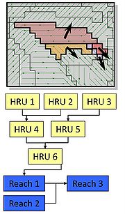
Hydrological Response Units (HRUs) are the modelling entities for the J2000 hydrological model. HRUs are 'saptial model entities which are distributed, heterogeneous structured entities having a common climate,land-use, soil, and geology controlling their hydrological dynamics' (Flügel 1995). The areas which comprise similar properties such as topography (slope, aspects), land-use, soil and geology, and behaves similarly in their hydrological response, are merged together to develop a HRU. The variation of the hydrological process dynamics within the HRU should be relatively small compared with the dynamics in a different HRU (Flügel 1995).
The processing of delineating HRUs are described in the following tutorial. GRASS-HRU tutorial. Users need to prepare the following file for HRU delineation.
- Digital Elevation Model (DEM)
- Soil
- Land-use
- Hydro-geology
All these data must be supplied in a raster format with a same resolution. The delineation of HRUs process provide HRU and Reach parameter files at the end.
- HRU parameter file (*hru.par)
| parameter | description |
|---|---|
| ID | HRU ID |
| x | easting of the centroid point |
| y | northing of the centroid point |
| elevation | mean elevation |
| area | area |
| type | drainage type: HRU drains in HRU (2), HRU drains in channel part (3) |
| to_poly | ID of the underlying HRU |
| to_reach | ID of the adjacent channel part |
| slope | slope |
| aspect | aspect |
| flowlength | flow length |
| soilID | ID soil class |
| landuseID | ID land use class |
| hgeoID | ID hydrogeologic class |
A sample HRU parameter file is provided below.
The HRU parameter file stores the spatial attributes of the catchment area where information about elevation, area, aspect, coordinates (x,y), land-use type (landuseID), hydrogeology(hgeoID) and soil(soilID) is stored for each HRU. The HRUs are topologically connected for lateral routing to simulate lateral water transport processes between an HRU to an HRU and was further connected to a nearby reach for reach routing. The column (to_poly) defines the HRU which passes water to next HRU.
The connection between the HRU parameter file and other parameter files is solved inside the HRU parameter file. For example, in the HRU parameter file, the HRU id 1 has all the necessary information as required in above table, including the land-use, soil and geology type which the HRU1 belongs to:
- Reach parameter file (*reach.par)
| parameter | description |
|---|---|
| ID | channel part ID |
| length | length |
| to-reach | ID of the underlying channel part |
| slope | slope |
| rough | roughness value according to MANNING |
| width | width |
The reach parameter file stores the information about stream characteristics as well as the relationship between stream networks to accomplish reach routing. The reach parameter file contains information on the structure of the flow topology by noting the ID for every reach into which it transfers. The reach parameter is produced along with the HRU delineation process and also comprises the information as required in above table.
With respect to the figure of the HRU parameter file above, the HRU ID 1 contributes water directly to REACH ID 1 whereas HRU ID 16 contributes water to HRU ID 5 which then contributes to REACH ID 2. The interactions between the parameter files were solved by a relation between the soil, land use and hydrogeological descriptors in the HRU parameter file and respective descriptors in the other parameter files.
Meteorological input data
The J2000 hydrological model requires the following input data for the model initialization:
| name | description | unit |
|---|---|---|
| ahum.dat | absolute humidity | g/cm3 |
| orun.dat | measured flow passage at the runoff | m3/s |
| rain.dat | measured amount of precipitation | mm |
| rhum.dat | relative humidity | % |
| sunh.dat | sunshine duration | h |
| tmax.dat | maximum temperature | °C |
| tmean.dat | mean air temperature | °C |
| tmin.dat | minimum temperature | °C |
| wind.dat | wind speed | m/s |
The J2000 modelling system uses Inverse Distance Weightings (IDW) with elevation correction method for the regionalization of the input climate data. The detailed description of regionalization approach is provided in:
[Regionalization approach of the J2000]
All the data as shown in above figure might not be available in some catchments. Normally, temperature and precipitaiton data are commonly available. In case, there are only few stations (less than 3) for some parameters, the IDW does not work properly. In that case, the same input value is applied for the entire catchment. For some particular variables, for example, temperature, this approach would bring larg amount of errors/uncertainties. In such cases, the regionalization approach based on a lapse rate is suggested for temperature. The details of this approach is provided in Nepal, 2012.
The relative humidity, wind and sunshine hours are also not frequently available in some catchments. These values are used for the estimation of evapotranspiration while using Pennman Monteith approach. The sunshine hours and wind speed can be assumed to be enough from one station, in case no other station data is available. In such cases, the same station value is applied for a whole catchment. The one station value for relative humidity also brings certain errors while calculating relative humidity using absolute humidity and temperature. In the J2000 modelling system, a direct regionalization of the relative humidity values is not recommended. The details are provided in 'calculation of evapotranspiration' sub-tutorial.
In case these data (rhum, sunh, wind) are not available the Pennmann-Monteith approach cannot be used. Rather a more empirical approach based on temperature such as Hargreves, can be used.
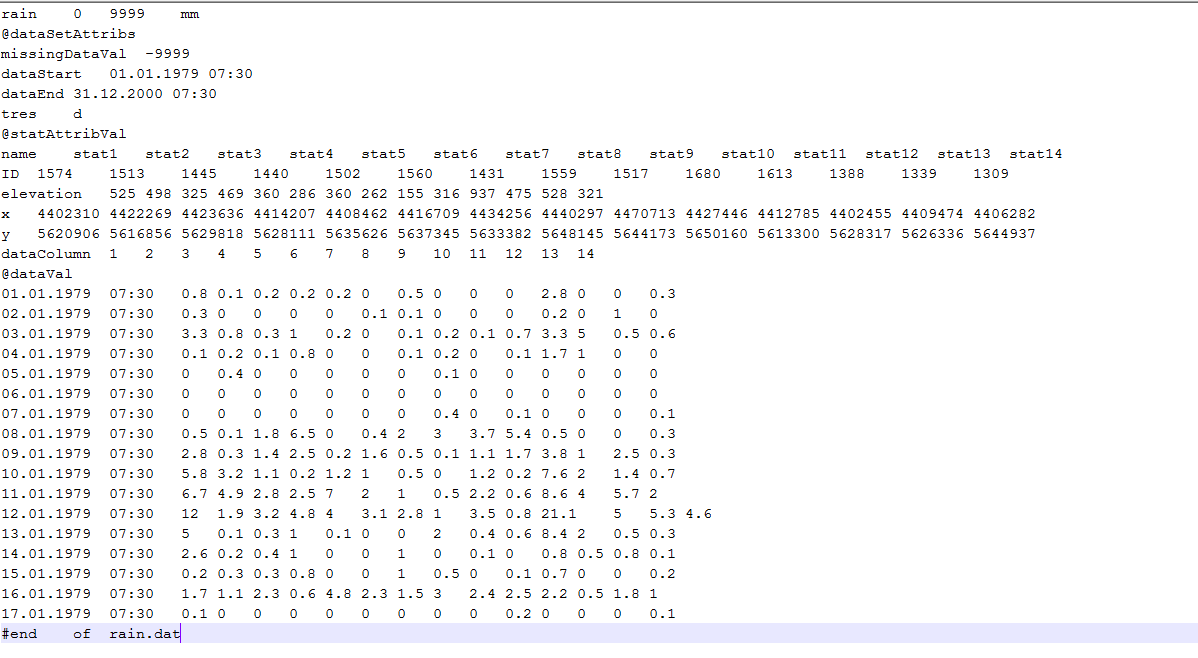
A sample of the Input data of rainfall (rain.dat) file is provided below:
The input data must be saved with extension .dat (example: rain.dat). The data in excel format can be saved as 'Text (tab delineated)(*.txt)' and changing the extention from *.txt to *.dat*. For more details, download the sample datafile:
Each data file has the following structure (demonstrated here for the example of rainfall):
| line | description |
|---|---|
| #rain.dat rainfall | |
| @dataValueAttribs | |
| rain 0 9999 mm | name of the data series, smallest possible value, biggest possible value, unit |
| @dataSetAttribs | |
| missingDataVal -9999 | value to mark missing data values |
| dataStart 01.01.1979 7:30 | date and time of the first data value |
| dataEnd 31.12.2000 7:30 | date and time of the last data value |
| tres d | temporal resolution of the data (here: days) |
| @statAttribVal | |
| name stat1 stat14 | names of the rainfall stations |
| ID 1574... 1309 | numeric id of the rainfall stations (ID) |
| elevation 525... 321 | elevation station1... elevation station14 |
| x 4402310... 4406282 | easting station1... easting station14 |
| y 5620906... 5644937 | northing station1... northing station14 |
| dataColumn 1... 14 | number of the particular column in the data part |
| @dataVal | beginning of data part |
| 01.01.1979 07:30 0.8... 0.3 | date, time, value station1... station14 |
| ... | |
| 17.10.2000 07:30 0.1..0.1 | date, time, value station1... station14 |
| #end of rain.dat | end of data part |
The input data of Dudh Kosi river basin can be downlaoded from here.
Workspace for input data
The input data of the J2000 hydrological model has to be provided in a specific folder considered as a 'workspace directory'. This workspace directory contains all the input data required to run the model and as well as the model output files.
Folders and files
The workspace directory has three main folders: input, output and parameters. The input folder has all the required input data to run the model. The parameter folder has parameter files (hru.par, hgeo.par, landuse.par, soil.par and reach.par). The output folder contains output files of different variables after the model is succesfully run. A sample workspace of testdataset is provided herewith which provides an idea of how to organise the workspace directory for the J2000 hydrological model.
Folder: input
The input folder has one 12 xml file of each input data. Please copy and paste these files as they are the connector for the real input data which are located inside the folder 'local'.
subfolder: local
The folder inside input folder contains the input data for eight variables (rain.dat, rhum.dat, sunh.dat, tmax.dat, tmean.dat, tmin.dat, wind.dat). The ahum.dat is created when the model is run first time by using the exisiting data.
subfolder: gis
Some GIS layers can be put here to display the spatial distribution of some output variables. For example, the spatial distribution of precipitaiton in a catchment (2D and 3D). For this, users need to put the DEM file of a catchment (data format: *.asc). The resolution of the DEM should be similar to the input DEM for HRU delineation process. Users need to copy the styles.sld file which is required to display a map. Additionally, HRUs, streams and station data files (*.shp) can be put in a seperate folder to display the variables in a map component. The name of these files and folders have to be defined in a model xml file [model xml file].
'subfolder: dump'
Create a folder with a name 'dump' which is used to dump temporary files.
Folder: output
The folder output has two xml files (HRULoop.xml and TimeLoop.xml) and a folder current. These *.xml file defines the variables for which the output is created.
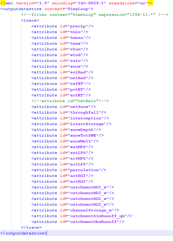
The TimeLoop.xml has daily output variables as shown in Figure below. If users do not need some variables, they can comment out the particular variables as shown in the case of netRain in the figure.
- HRULoop.xml file
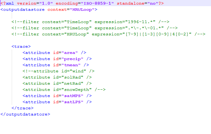
The HRULoop.xml is responsible for producing the daily average values of each variables of interest (as defined inside the xml file) for all HRUs. Users can comment out some variables as shown in the case of wind below.
- TimeLoop.xml file
Folder: parameter
The folder contains parameter files (hgeo.par, hru.par, landuse.par, reach.par, soils.par). Please remember that these names should be same in the model xml file.
Folders: explorer and tmp
The other folder inside the workspace is explorer and tmp which is used to dump some temporary files generated while running the model.
Model xml file
The workspace directory also contains a model xml file. The model files can be read as *.xml or *.jams. These model files are provided in example test dataset.
Definition of Model xml file: xx
Structure and example of a modules in terms of model source code.
The model xml file contains the logical structure of model framework and modules used in the model. It is organized in a systematic way that output from one module is supplied as input to the next module (example: snowmelt (output from snow module is an input for soil module). The model file also contains information about the display of different variables and outputs in the JAMS framework. The model xml can be viewed using the JAMS builder to understand the different component of a specific model.
Users can follow the following tutorial to get familiar with the JAMS Builder.
An example of Dudh Kosi model is provided in JAMS builder.
The left window shows the location of model source code files which are required to run a model. All the model source codes are inside the *.jar file. For the J2000 model, J2000.jar file is used. The middle window provides information about the modules used in the model xml file of the Dudh Kosi model. These modules are provided in logical structure where the output of one module is provided as input to next module. A detailed description of these different modules will be provided in later section. An example of Maximum temperature regionalisation module (TmaxLapseRate) is shown in the JAMS builder below. The module uses a single station temperature data to regionalize the maximum temperature in a catchment. By clicking the TmaxLapseRate in the middle column under Regionalization, the detailed information of the module is displayed in the right windows as shown in the figure below.
All the variables used in the modules are provided under the colum 'Name'. The colum 'Type' describes the characterisitcs of variables in terms of information (data, quality) they store in the variables. The column 'R/W' determines the input and output nature of the variables. Such as 'statElev' is a elevation of a temperature station which is denoted by R. This means the information is input to the module from preivous module and denoted by 'Read'. The 'W' denotes Write which is the new output value from this module. The calibration parameters, if any, are provided in the colum 'Value'. These information can be changed from JAMS builder instantly. Upon clicking the variable, the inforamation on 'attribute configuration' will be filled. These information can be changed. Please click 'set' to save the information.
The model can be run from JAMS builder by clicking the button 'Run Model' or 'Run Model from JAMS launcher' as denoted by green botton at the top banner. The latter will also provide a JAMS launcher from where users can change the different information (such as parameter values, time period)etc.
A more detailed description of model xml file in relation to different modules and vairables used in model source codes are described in (Krause, 2011). This document can be generated from the JAMS builder instantly. Click 'Model' from top banner and 'Generate Model Documentation'. The model documentation will be available in pdf format for download.
The model xml can be viewed and edited using text editor software also (such as PSPad) as shown below for the 'Maximum Temperature Regionalization module'.
<component class="org.unijena.j2k.regionalisation.TemperatureLapseRate1" name="TmaxLapseRate">
- This line defines the location of the module TemperatureLapseRate1 in the model library file *J2000.jar.
<var name="lapseRateWinter" value="0.6"/>
<var name="lapseRateSummer" value="0.55"/>
- The value of lapseRateWinter and and lapserateSummer is the calibration parameter which is a lapse rate of chagnge in temperature per 100 meter.
<var attribute="elevation" context="HRULoop" name="entityElev"/>
- The attribute elevation defines the elevation of an HRU which is input variable to the TemperatureLapseRate1 module. The model reads the elevation of each HRU from the HRU parameter file as explained earlier.
<var attribute="time" context="J2K" name="time"/>
- The time defines the temporal resolution of the model (eg. daily)
<var attribute="tmax" context="HRULoop" name="outputValue"/>
- tmax is the maximum temperature as output value from the module. It calculates a maximum temperature for each HRU using the input variables inside the module.
<var attribute="elevationTmax" context="J2K" name="statElev"/>
- elevationTmax is the input variable of elevation of maximum temperature station. The model read the elevation from the temperature station in input file (e.g. tmax.dat).
<var attribute="dataArrayTmax" context="J2K" name="inputValue"/>
- dataArrayTmax is the input variable of maximum temperature on a particular date.
<var attribute="tmaxOrder" context="HRULoop" name="statOrder"/>
- tmaxOrder defines the order of the station in case more than 1 temperature station is available based on the distance of an HRU with the temperature station. In that case, the model recognize the nearby station from the particular HRU.
The logical order of each variables used in the module is very important in the model xml file. For example, each input variables must be defined earlier before it is being used. For example, the input variable 'dataArrayTmax' is defined earlier in a module called 'TmaxDataReader' module. The module reads all the maximum temperature daily data in a format which the model can recognize. Similarly, the output variable 'tmax'(maximum temperature) is then used in a later section. For example: tmax (maximum temperature) value of each HRU is used to calculate snowmelt of that HRU.
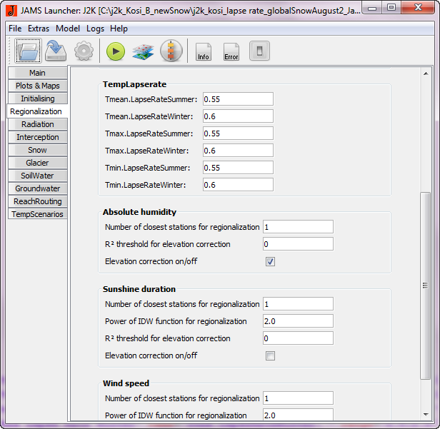
The calibration parameters (lapserate) can be defined in the initial part of the xml. It then can be displayed in the JAMS framework while running the model from where users can change the value. The figure below shows lines to display the summer and winter lapse rates for maximum, minimum and average temperatures.
- component (TmaxLapseRate) refers to the name of the module TemperatureLapseRate1 which is provded.
- range defines the range for the parameter which the models accept in the display part.
The figure below shows the calibration parameters for the lapse rate which is displayed in the JAMS framework. Users can change the value from the JAMS launcher.
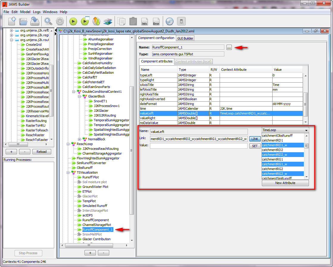
The xml file also contains components to display model results of certain variables. For this, the 'TSVisualization' component of the JAMS builder has to be expanded (click + and - sign on the left side to expand and reduce) as shown in Figure below. The existing TS plots will be shown. The new plot can be created by using the existing plot. Drag one of the existing plots (example, Glacier contribution) and hold CTRL key (a + sign will appear) and leave both the keys. The new plot will appear with the new name (Glacier contribution_1). From the right window, the name and the values of the new plot can be changed. Mainly, four things has to be changed in the new plot.
1. Change the name of the component. Click the [...] box on the right hand side of the 'Name'. This will bring a new window and you can change the name of the new plot.
2. Provide new names for the legend used in the plot. Click on the 'titleLeft' row and change the name of the legends under 'Value' window. In case of more than one legend, seperate the name by semicolon.
3. Provide colors to the legends. Click 'colorLeft' row and change the color name under 'Value' window.
4. Provide value for the legends. When 'valueLeft' row is clicked, the window below is activated. The value can be choosed from Timeloop. Use CTRL key to choose more than one value.
For this, the output variables must be defined in the TSPlot component at the end of an xml.
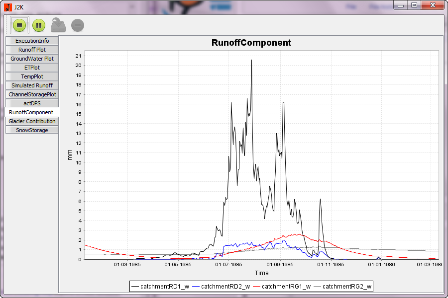
With these lines in xml file, users define which output files they wish to see as a plot/graph. In the figure below, four different runoff components are displayed.
After defining the plot, users also need to define a line in a 'Plot & Maps' component to bring it in the JAMS framework. For example: The first line is dedicated to display the Runoff plot.
The Runoff Plot will appear in Plots & Maps group in JAMS launcher after loading the xml file in JAMS, which users can tick on/off to display as a graph.
After running the model, users can see the graph of different runoff components as provided below:
Modules within the J2000 hydrological Model
This section describes the different modules within the J2000 hydrological model. The calibration parameters applicable to each module are also described with focus on their influence on streamflow. Following are the important modules in the J2000 hydrological model.
- Precipitation distribution module
- Interception module
- Snow module
- Glacier module
- Interception module
- Soil module
- Groundwater module
- Lateral routing
- Reach routing
Calculation of Evapotranspiration
[Calculation of evapotranspiration]
Precipitation distribution module
- Calibration parameters
| parameter | description | Global range | For Dudh Kosi model |
|---|---|---|---|
| Trans | threshold temperature | 0 + 5 | 2 |
| Trs | base temperature for snow and rain | -5 +5 | 0 |
These parameters are considered as non-flexible parameters and not necessarily placed in the JAMS framework as tunable parameters.
In the J2000 modelling system, the precipitation is first distributed between rain and snow depending upon the air temperature. Two calibration parameters (Trans, and Trs) are used where Trs is base temperature and Trans is a temperature range (upper and lower boundary) above and below the base temperature. In order to determine the amount snow and rain, it is assumed that precipitation below a certain threshold temperatures results in total snow precipitation and exceeding a second threshold results in total rainfall as precipitation. In the range (Trans) between those threshold temperatures, mixed precipitation occurs.
The detailed description of this module along with the algorithm as defined in the model source code is provided in: [Precipitation distribution module]
- Relevancies in modelling
Putting the Trs values below zero (e.g. 2) will bring more precipitation in the form of 'rain' than 'snow'.
Interception module
- Calibration parameters
| parameter | description | Global range | For Dudh Kosi model |
|---|---|---|---|
| α_rain | storage capacity (m²) of particular land cover for rain | 0 to +5 | 1.0 |
| α_snow | storage capacity (m²) of particular land cover for snow | 0 to +5 | 1.28 |
- Relevancies in modelling
Keeping the high value of α will store more water on leave surfaces which leads to higher evapotranspiration and less water available for runoff and vice versa.
Snow module
- Calibration parameters
| parameter | description | Global range | For Dudh Kosi model |
|---|---|---|---|
| snowCritDens | Critical density of snow | 0 to 1 | 0.381 |
| snowColdContent | cold content of snowpack | 0 to 1 | 0.0012 |
| baseTemp | threshold temperature for snowmelt | -5 to 5 | 0 |
| t_factor | melt factor by sensible heat | 0 to 5 | 2.84 |
| r_factor | melt factor by liquid precipitation | 0 to 5 | 0.21 |
| g_factor | melt factor by soil heat flow | 0 to 5 | 3.73 |

