Contents 1 Introduction in model calibration 1.1 Motivation 1.2 Requirements 1.2.1 Datasurvey 1.2.2 Choice of calibration parameters and definition of parameterarea 1.2.3 Specification of qualitycriteria and target functions 1.3 Identification of modellparameters 1.3.1 Äquifinality 1.4 Model Validation 1.4.1 Split Sample Validation 1.4.2 Cross Validation 1.4.3 Proxy Basin Test 1.4.4 Differential Split-Sample Test 1.4.5 Proxy-basin Differential Split-Sample Test 2 Calibration 2.1 Offline Calibration 2.2 Online Calibration 2.3 Operating OPTAS

Introduction in model calibration

Motivation

The modelation of hydrological processes is an challenging task: the investigated area can extend over a large scale of time and space. Hydrological processes proceed steady, in lots of different scales an depend on different variables. This variables interact with non linear complex correleations (Blöschl and Sivapalan, 1995).One independend process of the hydrological system is not sufficient enough for an analysis. It is necessary to have an allround understanding of the interaktions of the systemcomponents and - processes. This knowledge has to be gathered trough different diciplines. A lot of this processes proceed under the surface of the earth and are difficult to measure. Hydrological systementities can not be observed in there full connection, because the measured data is not fluent and has to be determined discretely.

This is aspecially difficult for systemconditions, because they are very variable in there time and space. Representative measured data is very time-consuming in there acquisition (Wainwright and Mulligan, 2004).

This is why the components of all hydrological modells are partial conceptional descriptions of processes in reality (Crawford and Linsley, 1966). Although this fact was determined 45 years ago, it is still up to date (Duan et al., 2003). As an consequence can a lot of modellparameters not be determined directly, because they haven't an direct physical connection or there werent any measurements (Gupta et al., 2005). That is why the parameters are determined indirectly, by searching for an modellparametrition. This leads to an best possible adjustment of the simulation in the natural system. For an successfull usage of the modells is an carefull determination of the modellparameters essential. In the most time are the modellresults not in an linear correlation with the modellparameters and the basic used modells arent analytical usefull. This is the reason why most time can not be used direct solvatioan methods. The parameters have to be determined by "trial and error" processes (Gupta et al., 2005).

A special role fullfill the unmeasured riverflowareas or areas with very only few datas, in the callibrationprocess. The callibration can not be done directly in this case. Modells with an strong physical basis(Koren et al., 2003), or statistical analysis (e.g. Jakeman et al. 1992;Wagener et al. 2004), or both methods combined are used to overcome this problemes. Strong physicalbased modells can determine a lot of parameters, by direct measurement or empirical equations based on the propertys of the area. The statstical analysis develops an connection between parametervalues and the propertys of the area. Models of unmeasuered FEG will not be considered in this thesis. So that the calibration on observed systemconditions can be narrated.

Requirements

Precalculation decitions must be made, in dependence on the modelltask. Therefore Grundmann (2009) states;

1. Selection of Data, that should be used
2. Selection of definitions and to callibrated parameters in the parameterspace
3. Specification of excellencecriteria and target function
4. Selection of optimizing strategie
5. Selection of strategie for validation and insecurity analysis

Datasurvey

For an succesfull callibration is it necessary to check the the data in regard of consistency and homogenity (Grundmann, 2009). The calibration can be done with different observations. There are plenty of thesis of groundwater measurements (Blazkova et al., 2002; Madsen, 2003), the snowcoverage (Bales and Dozier, 1998),ground humidity (Merz and Bárdossy, 1998; Western and Grayson, 2000; Scheffler, 2008) and evapotranspiration (Immerzeel and Droogers, 2008). But in the most cases are the hydrological modells callibrated with the measuered drainflowlines (Seibert, 2000). The reasons therefore are: (i) a lot of waters have an longtime draintimeline, (ii) the drain is an aggregated signal for most of the relevant hydrological processes of the river-drainage-basin, with (iii) relatively small measuringerrors and (iv) an high repeat value. Therefore is the calibration often done with the drainage-course-line.

Choice of calibration parameters and definition of parameterarea

The question for the selection of parameters to calibrate isnt trivial at all. It depends from the to calibrating model and his application. A lot of hydrological modells own more parameters than can be calibrated. Therfore should only be the parameteres calibrated that can't be directly determined (e.g. from the landscape attributs) and that have significient impact on the modellbehavior. The identification of those parameters can be done by an sensitivity analysis of the modell. This provides not only information about the quantitiy effect of the paramerters, as well as an big help for understanding the modell (Saltelli et al., 2008).

Often is the definition of parameterborders not obvious either. Depending on the grade of physical connections can critical values and matching standard values of the parameters be: (i) evaluated directly through measuring (in labor conditions or real systems), (ii) determined from plausible-considerations or (iii) from experienced - literaturvalues transfered. Often provide modelldocumentations a choice of parameterborders (see e.g. DYRESM (Hamilton and Schladow, 1997), J2000(Krause, 2001), WaSim-ETH (Schulla and Jasper, 2000)). This borders have an large range , because they have to reflect the initial uncertainty of the parameters when knowledge about the modellusage is missing. An introduction of callibrationparamerers of the modells: J2000 and J2000g can be found here and here.

Specification of qualitycriteria and target functions

The task of the calibration is it to reduce the parameter uncertainty step by step to an minimum. For this optimization is it necessary to compare evaluations of the simulated hydrographs. Although it is the best method to examine the hydrograph bye an expert, for judging the performance of the modell (Krause et al., 2005), it is necessary to have an mathematical errorfunction for an objective quantifiable evaluation. Errorfunctions represent the part of measured data, that could not be reproduced by the modell. It is possible to classify in absolute and relative errorfunctions. Relative errorfunctions have the advantage of beeing dimensionless, that means they can be compared overall applications. Errorfunctions, that are often used in the context of hydrologie, are p.e. the Nash-Sutcliffe efficience (Nash and Sutcliffe, 1970) and there modifications, the determinationrate and the absolute - relative voluminaerror (Krause et al., 2005).

Krause et al. (2005) get to the conclussion by the comparisson of multiple errorfunctions, that none of the ratios shows all relevant aspects of an hydrograph. They get to the conclussion that every errorfunction has its own specific pro and cons. Although there where a lot of errorfunction proposed that counter the deficits, there hasn't been an anwser for the universal ratio. An overview about the different errorratios and there characteristica can be found here.

Identification of modellparameters

The search for fitting parameterdata can be done manuell or automaticaly. The manuell possibility can lead to excellent results, but it is hard and connected with a lot of worktime, personal, costs and is tied to subjectiv processdecisions (Boyle et al., 2000). An alternativ is the automatic callibration with its mathematical optimizationprocesses, that can solve quick and objectiv complex problems.

In the past was the automatic callibration done with local optimizationprocesses, like the gradientdescent. It was fast recognized that on this way it is not possible to discover optimal parameterdata reliabely. Because of a lot unfitting properties with this method (Duan et al., 1992). Therefore developed Duan et al. (1992) the Shuffled Complex Evolution (SCE) method, which proved itself in the last 20 years as very robust, efficient and effectiv. Thats why it is used until today in terms of hydrological themes (p.e. Sorooshian et al. 1993, Eckhardt and Arnold 2001, Liong and Atiquzzaman 2004).

General shouldnt be the calibration understood as an method to finde parameterdata, that will be used to adapt the modell to the surveied data (Vidal et al., 2007); rather it is an continuous process of the parameteridentification. Therefore is the initial insecurity reduced step by step; by reducing the parameterarea to the parameterdata, that leads to the modellbehaviour, which is qualitativ and quantitativ consistent in terms of the systembehaviour. There cant be an hundred percantage conformance of the modell and reality. Because every modellstructur and parametrization is an approximation of the real systemstructur and every modellprediction is affected with an insecurity. Gupta et al. (2005) characterizes an calibration of an hydrological modell as:

1. The input/output of the model is consistend with the observed drainagearea behaviour. 2. The modelpredictions are accurate (that means they have an insignificiant system error) and exact (that means the insecurity of the predictions are low) and tough. That means, little changes of parameters result in little model changes. 3. The model structure and model behaviour are consistent with the actual hydrological behaviour of the real system.

Äquifinality

The identification of modelparameters from an impuls/anwser-behaviour is known under the term: inverse problem or identificationproblem (Cobelli and DiStefano III., 1980) and is not only a term of hydrologcal context. Inverse problems are often bad posed (Kabanikhin, 2008), that means they have neither a solution or infinit solutions or the the systems behaves chaoticaly. Bellman and Astrom (1970) could demonstrate formal, that inverse problems aren't resolvable in very easy systems either, if there aren't every intern conditions of the system observable. That means for hydrological modeling that the systembehaviour can be explained by different models with different structures and parameterization. For this phenomenon has Beven (1993) defined the term of Äquifinality, which has its origin from Ludwig von Bertalanffy (Von Bertalanffy et al., 1950). Äquifinality is the term, that the provided information doesn't last to descripe the system completly. Wagner and Gupta (2005) differentiate in three philosophies about the handling of Äquifinality:

• Parsimonie: Äquifinality or parameter-insecurity can be an hind, that the chosen modelstructur is to complex in terms of data. The source of this philosophie is the observation, that easy, less data intensiv models provide often better predictions then complex, physical based models (Loague and Freeze, 1985;Reed et al., 2004). Thr principle of parsimonia tells, that always should be the easyiest explanation used for an phänomenon. Even Aristoteles represented this principle and it was postulated by William of Occam at the beginning of the 14 century. Therfore is the term "Occam's Razor" common. Following this rule, should there be the structure of hydrological model's be as easy as possible and only be added with complexity when the precision of the model doesn't fit the intended cause. Multiple papers show, that the parameter insecurity can be lowered by the reduction of modelcomplexity (Jakeman and Hornberger, 1993; Weater and Jakeman, 1993; Young et al., 1996; Wagener et al., 2002,2003b).

• efficient information usage: Traditionally will be only one objective criteria used for the calibration. By this one-criteria optimization will be the simulated and real drainage compared and reduced to only one numeric data, out of thounds of data sets. This information-loss is for Gupta et al. (1998) an reason for appearnce of Äquifinality . There are two ways of reducing the information-loss: first, agrumentated Gupta et al. (1998), that the search for optimal parametric data sets an multicriteria probleme by itself is. The multi-criteria optimization considers at the calibration multiple objective criteria simultaneously. As an result is therean muliple amount of information that counters äquifinality. That is why this way has been very popular in the last ten years. The second way is to extract the information in the data by sub dividing the amount of data. Methods, that can be used are the Kalman filter and its extansions (Kitanidis and Bras, 1980), PIMLI (Vrugt et al., 2002), BARE (Thiemann et al., 2001) and DYNIA (Wagener et al., 2003a).

• acceptance of äquifinality: Äquifinality can be regared as an inherent propertie of the problem. The logical consequenzes are to to keep all potential solutions of the callibration problem and involve them into modelation, as long as they can not be separeted because of other reasons. This ensemble of solutions can be used, p.e. for analyzis of parameter insecurity with the Generalized Likelihood Uncertainty Estimation Method (GLUE, Beven and Freer 2001) or DREAM (Vrugt et al., 2008).

The treatment of the äquifinality is tied closely to the consideration of model insecurities. Hydrological models have often there usage in critical systems, like the prediction of natural disasters, the prediction of longtime inffluences of climatic change or the development of adaptionstrategies of the water-infrastructure. Therefore is the estimation, preparation and communication of model insecurities and the borders of model predictions very important from the point of our society (Montanari et al., 2009).

Model Validation

The model validation serves as evidence for the suitability of a model for a certain intended purpose (Bratley et al. 1987). Model validation is an important tool for quality assurance. A model is useful for implementation if it proves to be a reliable representation of real processes (Power 1993). Different key figures and proofs may be required subject to the purpose and type of model in order to validate the model.

In general, there are different quality criteria which play a role for model validation:

• Accuracy/precision: The accuracy of a model represents the deviation of simulated values in comparison to real (measurement) values. This is mostly quantified by the Nash-Sutcliffe efficiency, degree of determination or mean square error.
• Uncertainty: The input values of an environmental model often contain errors and uncertainties. In addition, there is no complete knowledge regarding a natural system, i.e. the modeling has uncertainties. The impact of these values is quantified by the insecurity of the model, i.e. the uncertainty reveals the confidence interval of a model response.
• Ruggedness: The ability of the model to maintain its function if there are (minor) changes in the natural system (e.g. change of land use in a catchment area). This is closely linked to
• Sensitivity: which indicates the influence of (minor) changes in the input data and model parameters on the result
• Validity: is the property of the model to provide correct results for the right reasons, i.e. the explanation for a system which is given by the model is correct.

The following methods for the validation of hydrological models were put forward by Klemes (1986).

Split Sample Validation

The amount of validation data which is available (e.g. runoff time scales) is split into two sections. First, section 1 is used for calibration and section 2 for validation of the model. Then the calibration part and the validation part are swapped. For this reason both section should have an equal size and provide a for adequate calibration. The model can be classified as acceptable if both validation results are similar and have sufficient properties for model application. If the available amount of data is not large enough for a 50/50 division, the data should be split in such a way that one segmaent is large enough to carry out a reasonable calibration. The part remaining is used for the validation. In this case the validation is supposed to be carried out in two different ways. For example, (a) the first 70% of the data are used for calibration and the remaining 30% for validation, (b) then the last 70% of the data for calibration and the remaining first 30% for validation.

Cross Validation

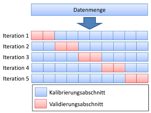
Cross validation is a further development of the split sample test. The amount of data is split up into n sections of equal size. Now n − 1 sections are used for the calibration and the remaining part is used for validation. The amount for the validation is swapped, so every set of data is validated once. This method requires much more computational effort than the split sample validation but it has major advantages if there is a small amount of data and it allows for a validation of every kind of data set. A special case of this validation is the Leave-One-Out Validation (LOO). It always uses exactly one data set for validation and the remaining part for validation. Due to the huge effort this kind of validation is mostly applied in special cases.

Proxy Basin Test

This is a basic test concerning the spatial transferability of a model. If, for example, the runoff is supposed to be simulated for a non-measured area C, two measured areas A and B can be selected within a region. The model should be calibrated with data from area A and validated using data from area B. Then roles of area A and B should be exchanged. Only if both validation results are acceptable with regard to modeling application, it can basically be assumed that the model is able to simulate the runoff of area C. This test should also be applied if an amount of data is available for area C which is not sufficient for the split sample test. The data set in area C would not be used for mode development but only as an additional validation.

Differential Split-Sample Test

This test should always be used if a model is supposed to be applied under new conditions in a measured area. The test may have several variants, subject to the way in which the conditions/properties of the area have changed. Those changes include, for example, climate changes, changes of land use, the construction of building, which influence the hydrology in the region etc.

For the simulation of effects of climate change the test should have the following form. Two time periods with different climate parameters should be identified in historical data sets; for example, a time period of high mean precipitation and another period of low precipitation. If the model is supposed to be used for runoff simulation of humid climate scenarios, the model should be calibrated with the arid data set and the validation should be carried out with the "humid" data set. If it is supposed to be used for the simulation of an arid scenario, the procedure should be reversed. In general, the validation is supposed to test the model under changed conditions. If no sections with significantly different climatic parameters can be identified in historical data, the model should be tested in another area where the differential split-sample test can be carried out. This is mostly the case if not climate changes but, for instance, changes of land use are considered. In this case a measured area has to be identified where similar changes of land use have taken place. The calibration should be carried out using original land use and validation using the new land use.

If alternative areas are used, at least two areas of such kind should be identified. The model is calibrated and validated for both areas. The validation can only be successful if results for both areas are similar. It has to be noted that the differential split-sample test, in contrast to the proxy - basin - test, is carried out for both areas independently.

Proxy-basin Differential Split-Sample Test

As the name suggests, this test is a combination of proxy-basin and differential split-sample test and it should be used if a model should be transferable in space and is applied under changed conditions.

Calibration

There are two common methods for calibrating a model with the integrated Standard Efficiency Calculator.

Offline Calibration

First, it is possible to carry out a calibration locally on your own computer. However, this uses computing resources for a longer period of time.

Step 1

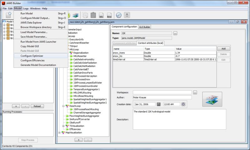
Open the JAMS User Interface Model Editor (JUICE). Load the model you want to calibrate. The following window should appear:

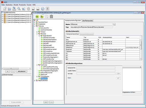
Step 2

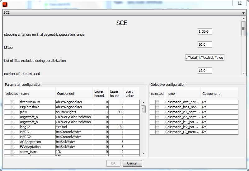
Select now the tab Model and click on the option Configure Optimizer. There should be now alogwindow that enables the configuration of your calibration (see picture below).

Step 3

In the upper part is a tap that can set the typ of your optimization process that will be used in the calibration. At the moment the following methods are available: + Shuffled Complex Evolution

• Branch and Bound
• Nelder Mead
• DIRECT
• Gutmann Method
• Random Sampling
• Latin Hypercube Random Sampler
• Gauß Process Optimizer
• NSGA-2
• MOCOM
• Paralleled Random Sampler
• Paralleled SCE

For the application with single target criterion the Shuffled Complex Evolution (SCE) and DIRECT are recommended. Most probably both find a global optimized parameterization. It has been attested that DIRECT shows robust operation and no parameterization is necessary. SCE only needs one parameter: the Anzahl der Komplexe (number of complexes). This parameter indirectly controls whether the parameter search area is browsed rather broadly or if the process quickly concentrates on a (sometimes local) minimum. In most cases, the default value 2 can be used. For multi-criteria optimization NSGA - 2 seems to provide very good results. However, there are more detailed analyses to be carried out. We will use in our example SCE.

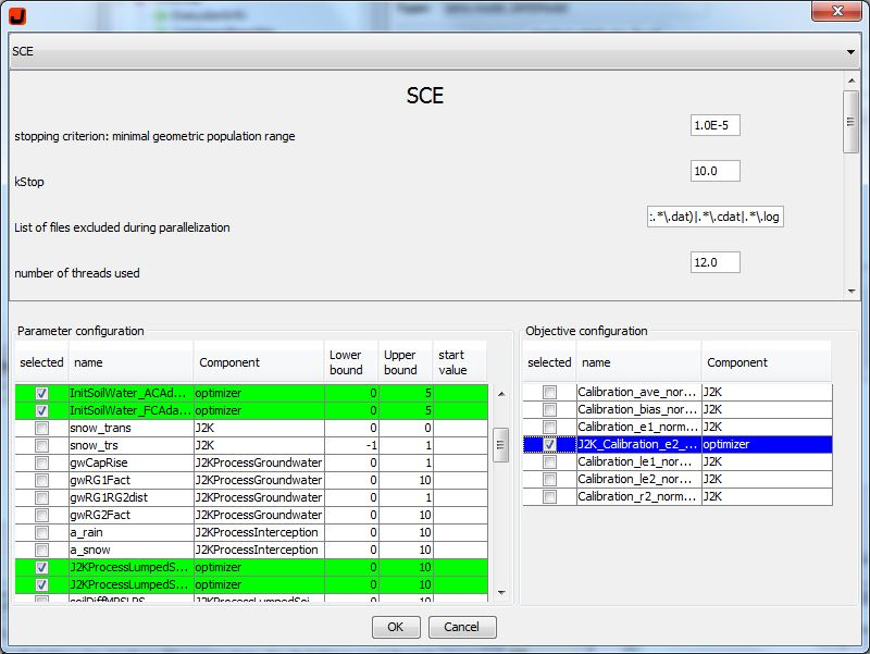
In the middle of the dialog area, on the left hand side, are the potential parameters of the model are listed. Select those parameters from the list which you want to calibrate. If you want to select more than one parameter, hold down CTRL while selecting the parameters. Now you can see several input fields for each parameter on the right hand side. You can choose the lower and upper bound which define the area in which the parameter can vary. In addition, it is possible to define a start value. This makes sense if a parameter is already known which suits as a starting point for the calibration.

Step 4

On the left-lower side of the Window is the parameterkonfiguration. There you can select the parameters you would like to optimize. If you want to you can change the Lower and Upper limit or, if you have specific data, you can set a start value. Caution: If you set one start value, you have to set a start value for all your selected parameters! At the moment it is not possible to set a start value for one parameter and leave the other parameters with a Lower and Upper limit. There has to be an start value or lower and upper limit for every selected parameter.

Step 5

The preset efficiencies, from "Set Evaluation criteria", should be in the right lower part of your window. You can select them individually to set your optimization for your use.

Step 6

When you are ready with your settings, you can press the OK button to start the optimizationprocess. Your window will close and the program should return to your JAMS Builder window. Now you can start the Optimization by clicking on the Run Model button. You will see the ongoing optimizationprozess in the lower left side at Running Processes.

Online Calibration

As an alternative to offline calibration the process can be carried out on the computing cluster of the Department of Geoinformatics, Hydrology and Modelling at the Friedrich - Schiller - University Jena. This does not occupy any local computing resources and allows a calibration of up to four models at the same time.

Step 1

Open your Internet browser (e.g. Firefox) and go to website [[1]] You will now see the following window and you will require a login. In order to register please contact

• Christian Fischer
• christian.fischer.2@uni-jena.de

Step 2

After the registration you will see the main window of the application.

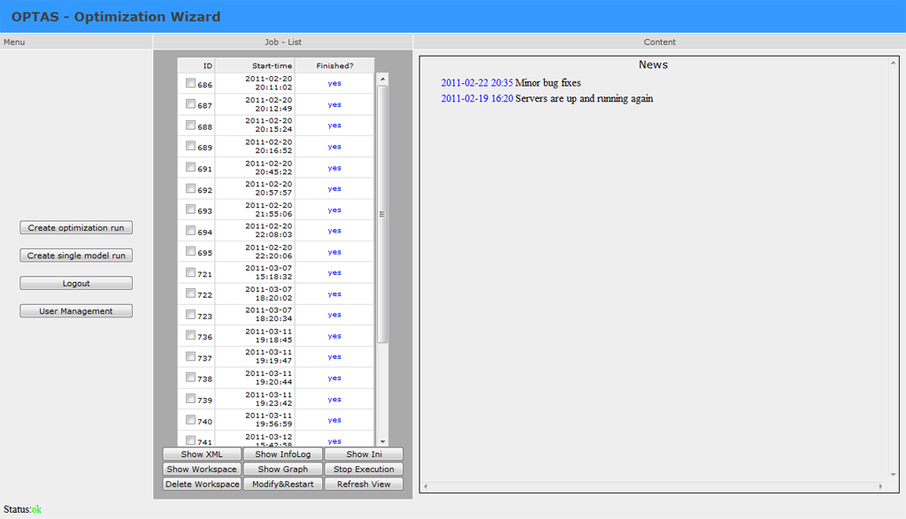
The window is split up into three parts. In the middle you can see a list of all tasks that have been started. All tasks which have been finished are marked in blue color and tasks which are being carried out are marked green. Red entries indicate that an error has occurred during the configuration of a new task/calibration. The right part of the window shows different contents. When starting the application, you can see news about the OPTAS project. In general, information up to a size of 1 megabyte is shown. Greater data sizes are not shown because it affects the page view. Instead, a zip file is created from the information which is then available for download.

Step 3

In order to carry out a new calibration, click on "Create Optimization Run". You will now see the first step of the calibration process.

In this step you will be asked to enter the data which is necessary. Load the model for the calibration (jam file) into the first file dialog. Pack your working directory of the model as a zip archive. A suitable programs is for example 7-zip. Please note:

• the working directory cannot be in a subfolder
• please do not load any unnecessary files (e.g. in the output file). The upload is limited to 20mb.
• the file default.jap is not allowed to be in the working directory

Now load the packed working directory into the second file dialog. The modeling will usually be carried out by using the current version of JAMS/J2000. Libraries for J2000g and J2000-S are usually available as well, so you will not need any files for most applications.
Should you need any versions of component libraries which are particularly adapted for models J2000, J2000-S or J2000g, please load them (unpacked) into the corresponding file dialogs. If your models requires additional libraries, you can indicate them as a zip archive in the corresponding file dialog. To finish, click on Submit. The files that you indicated are now are now being loaded on the server environment. The management server (sun) checks the host for free capacities and assigns a host to your Task.

Step 4

After transferring the model and the workspace, the following dialog for the selection of parameters and goal criteria appears.

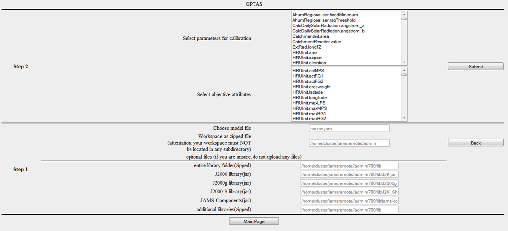
The first list shows all potential parameters of the model. Select those parameters which you want to calibrate. If you want to select several parameters, hold CTRL when marking them. In the low part of the dialog a target function is specified. You can either select a single criterion or several criteria (hold CTRL). When selecting several criteria, a multi-criteria optimization problem is created which differs significantly from a (common) one-criteria optimization problem regarding its solution characteristics. Since not every optimization method is suitable for multi-criteria problems, not all optimizers are available in this case.

Step 5

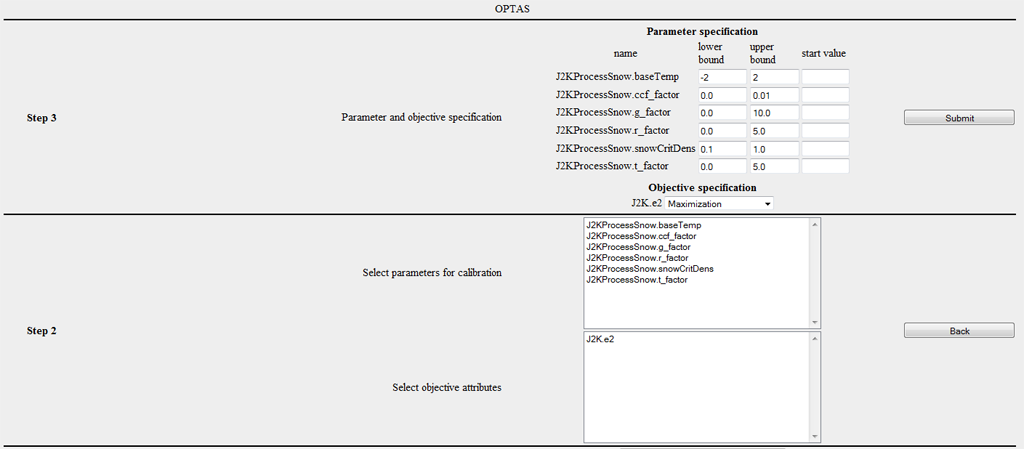
In this step, the valid range of values is to be specified for every parameter. For every selected parameter an input field is available for the specification for upper and lower boundaries. The fields are occupied by default values, if they are available for the specific parameter. These default values are mostly very broad, so it is recommended to carry out further restrictions. In addition, there is an optional possibility to indicate the start value. This is helpful if an adequate set of parameters is already available which is taken as the starting point of the calibration.

In the second part, you can choose for every criterion whether it should be

• minimized (example RSME - root square mean error),
• maximized (example r²,E1,E2,logE1,logE2),
• absolutely minimized (i.e. min |f(x)| e.g. for absolute volume error),
• or absolutely maximized.

The following image shows the corresponding dialog. In this example, the parameters of the snow module were chosen and the default thresholds were entered.

Step 6

You are now asked to choose the desired optimization method. At the moment, the following methods are available:

• Shuffled Complex Evolution (Duan et al., 1992)
• Branch and Bound (Horst et al., 2000)
• Nelder Mead
• DIRECT (Finkel, D., 2003)
• Gutmann Method (Gutmann .. ?)
• Random Sampling
• Latin Hypercube Random Sampler
• Gaußprozessoptimierer
• NSGA-2 (Deb et al., ?)
• MOCOM ()
• Paralleled random sampling
• Paralleled SCE

For most one-criterion applications the Shuffled Complex Evolution (SCE) method and the DIRECT method can be recommended. For multi-criteria tasks the NSGA-2 mostly delivers excellent results.

Step 7

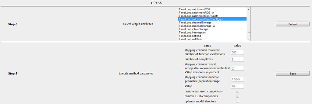
Many optimizers can be parametrized according to the specific task. SCE has a freely selectable parameter: the number of complexes. A small value leads to rapid convergence, though with higher risk of not identifying the global solution, whereas a greater value increases calculation time significantly while strongly improving the possibility of finding an optimum. Mostly a default value of 2 can be used to work with. In contrast, DIRECT for example does not possess any parameters. It shows a very robust behavior and no parametrization of the method is required. Moreover, three check boxes are available which are not subject to the specific method.

• remove not used components: removes components from the model structure which definitely do not influence the calibration criterion
• remove GUI-components: removes all graphical components from the model structure. This option is highly recommended since e.g. diagrams influence the efficiency of the calibration in a very negative way
• optimize model structure: at the moment without function

The following image shows step 7 for the configuration of the SCE method.

Step 8

Before starting the optimization you can indicate which variables/attributes of the model should appear in the output. As a default, those parameters and target criteria are shown which have already been chosen which makes manual selection unnecessary. Pleas note that saving temporally and spatially varying attributes (z.B. outRD1 für jede HRU) may require a huge amount and this may exceed the size belonging to a user account.

Step 9

You now receive a summary of all modifications which have been carried out automatically. Particularly, you now have a list of components which are classified as irrelevant. By clicking on Submit you start the optimization process.

Operating OPTAS

After having started the calibration of the model, you should now see a new job on the main page. This is shown green to indicate that the execution is not yet completed. You also see the ID, the start date and the estimated date of completion for the optimization. If you select the generated job, you now have various options at your disposal.

Show XML

You can see the model description for carrying out this job which has automatically been generated. As soon as you click on the button, it appears on the right hand side in the window and can be downloaded from there as well.

Show Infolog

Click on this button in order to view status messages of the current model. When using an offline execution of the model this information is written in the file info.log or error.log.

Show Ini

The optimization-Ini file contains all settings applied and summarizes them in abbreviated form. This function is meant for the advanced user or developer, hence there is no further explanation at this place.

Show Workspace

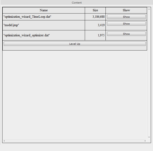
This function lists all files and directories in the workspace. By clicking on the directory/file its content is shown. The modeling results can usually be found in the file /current/ which is shown as an example in the following image.

It is to be noted that file contents can only be represented up to a maximum size of 1 megabyte and they are otherwise zipped in a zip file and made available for download.

Show Graph

Dependencies between different JAMS components of a model can be graphically displayed. This function generates a directed graph the node of which is the number of all components in the model. In this graph, a component A is linked to a component B if A is dependent on B, in the sense that B generates data which are directly required from A. Moreover, all components are shown red which have been deleted during model configuration. This dependency graph allows for an analysis of complex dependency relations, as for example the determination of components which are indirectly dependent on a certain parameter. Such kinds of analyses should, however, not be carried out. The graphical output of this graph is primarily used for visualization.

Stop Execution Stops the execution of one or more model runs.

Delete Workspace Deletes the complete workspace of the model on the server environment. Please use this function when the optimization is completed and when you have saved the data. This discharges the server environment and accelerates the display of the OPTAS environment.

Modify & Restart This function is addressed to advanced users. Often a restart of a model or calibration task is required without further need of modifications in the configuration. By using the function Modify & Restart the configuration file of the optimization can be directly changed and afterwards the restart of the model can be enforced in a new workspace.

Refresh View Updates the view. Please do not use the update function of your browser (usually F5) since this leads to a re-execution of the last command (e.g. starting the model).