The tutorial is prepared to use the J2000 hydrological model for hydrological system analysis of a river catchment. A test dataset of the Dudh Kosi river basin have been provided along with the tutorial. The Dudh Kosi river basin was used for the hydrological system analysis by using the J2000 hydrological model as a part of the PhD research (Nepal, 2012). The information provided here is largely based on this study [PhD Thesis]. Users can use the test data to get familiar with the model application. At the same time, users can prepare their own dataset to simulate the hydrological behavior of any catchment by following this tutorial. A separate section is provided at the end of the tutorial to use the J2000 model for a new catchment. [How to set up a new model]. Similarly, the information about the users forum for the Integrated Landscape Management System (ILMS) application is also provided at the end which can be used as a discussion forum to discuss issues related to the modelling application. Via the forum, the model developers and users can be reached.

The different components of the ILMS software (ILMSimage, ILMSgis, ILMSmodel, and ILMSexplore) from here. This tutorial explains how to download the ILMS software package.

Contents 1 Who can use the tutorial 2 Description of the test dataset 3 The J2000 model 4 Dataset preparation 4.1 Model parameter files 4.1.1 Soil parameter file 4.1.2 Land cover parameter file 4.1.3 Hydro-geological parameter file 4.1.4 HRUs and Reach parameter files 4.2 Meteorological input data 4.3 Workspace for input data 4.3.1 Folders and files 4.3.2 Model xml file 5 Display model results and output 6 Modules within the J2000 hydrological Model 6.1 Calculation of Evapotranspiration 6.2 Precipitation distribution module 6.3 Interception module 6.4 Snow module 6.5 Glacier module 6.6 Soil water module 6.7 Groundwater module 6.8 Routing module 7 Model calibration 8 Setting up a new model 9 Discussion Forum

Who can use the tutorial

The tutorial is prepared in such a way that the J2000 hydrological model can be used independently without any techtical support from model developers. Therefore, it can be used by students, model developers and researchers for the hydrological system analysis of a catchment. The tutorial should be read in conjunction with other sub-tutorials which has been mentioned in different part of this tutorial. Additionally, the tutorial is supplied with test dataset of the Dudh Kosi river basin (Nepal, 2012) which users can use to get familiar with the different aspects of the J2000 model. Similarly, users can also create their own dataset of the catchment of interest to run the model.

Description of the test dataset

The tutorial is accompanied by the test dataset of the Dudh Kosi river basin. The Dudh Kosi river basin is a sub-catchment of the Kosi river basin, Nepal located in the Himalayan region. The Department of Hydrology Meteorology (DHM), Government of Nepal, collects and manage the hydro-meteorological data. Six precipitation and one climate station is available in the Dudh Kosi river basin. Since, the measured data is not allowed to distribute publicly, the data provided here is not from the real stations. These data are from virtual stations in which the data the regionalized data were used and further processed with random errors. These input dataset are provided below along with the workspace directory to run the J2000 model. The users are expected to use the tutorial along with the test data to understand different aspects of the J2000 modelling system and also aim to prepare their own datasets to run the model. Users should contact the DHM Nepal directly to get the real observed data from the stations. The modelling results with the measured data from DHM, Nepal can be found in the PhD dissertation (Nepal, 2012).

To understand the motivation, objectives, methodological approach and the study area adopted for the hydrological system dynamics of the Dudh Kosi river basin, the PhD thesis can be referred for further details.

The J2000 model

The J2000 model is a distributed and process oriented distributed hydrological model for hydrological simulations of meso-and macro-scale catchments. It is implemented in the Jena Adaptable Modelling system (JAMS), which is a software framework for component-based development and application of environmental models (Kralisch and Krause 2006, Kralisch et.al. 2007). The simulation of different hydrological processes is carried out in encapsulated process modules which are to a great extend independent of each other. This allows changing, substituting or adding single modules or processes without having to restructure the model once again from the start. With this flexibility, a glacier module is integrated as a part of the study carried out by Nepal (2012) in the Himalayan region.

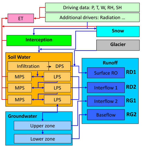
The modelling application represents the important hydrological processes of a river catchment. The principal layout of the J2000 hydrological model is provided in the figure below. The layout also includes the glacier module which has been applied in the Himalayan region. The modelling system differentiates among four different runoff components according to their specific origin. The component with the highest temporal dynamics is the fast direct runoff (RD1) (overland flow). It consists of the runoff of sealed areas and surface runoff originating due to saturated access and infiltration access runoff. The slow direct runoff component (RD2) (also known as Interflow 1), which corresponds to the lateral hypodermic runoff within soil zone, reacts slightly more slowly. This process reacts slightly more slowly than RD1. Two further base flow runoff components can be distinguished. The relatively 'fast baseflow runoff (RG1) (also known as Interflow 2) simulates the runoff from the upper part of an aquifer, which is more permeable due to weathering, compared to the lower zone of the aquifer. The slow baseflow runoff component (RG2), which can be seen as flow within fractures of solid rocks or matrix in homogeneous unconsolidated aquifers.

The detailed description of the modelling systems is provided in many publications. Some of the important publications are: (Krause, 2001,; Krause 2002,; Krause, 2010,; Nepal, 2012; Kralisch and Krause 2006,; Kralisch et.al. 2007). Some of the publications can be also accessed from this link: http://jams.uni-jena.de/index.php?id=5582&L=2

Dataset preparation

Model parameter files

The requirements of the data to run the J2000 hydrological model is discussed in detail here. Two types of data are required i) model parameter files and ii) meteorological input data. The first one is prepared and quantified inside the GIS environment and known as model parameter files. The parameter files and their values are static in the modelling application.

Users have to prepare all the input data (i.e. soil, land cover, geology, DEM) in raster format with certain resolution. While delineating HRUs, all the input data has to be provided in the same resolution. The resolution of the dataset mainly controls the number of HRUs to be formed without losing the heterogeneity of a catchment. Therefore, the resolution of input data depends upon the catchment to be modelled. For example, if the catchment is small (e.g. 1000 km²), the resolution between 30-90 is suitable depending upon the resolution of the available dataset. Similarly, for meso-scale catchment (e.g. 4000 km²), resolution between 250-500 m is suitable. In addition, a catchment with flat topography (e.g. low gradient) needs fine resolution data to characterise the features of a catchment.

The detailed descriptions to derive the parameter files are provided below:

Soil parameter file

The detailed information required for the soil parameter file is provided in Table below.

Parameter	Description
SID	soil type ID
depth	soil depth
kf_min	minimum permeability coefficient
depth_min	depth of the horizon above the horizon with the smallest permeability coefficient
kf_max	maximum permeability coefficient
cap_rise	Boolean variable, that allows (1) or restricts (0) capillary ascension
aircap	air capacity (equivalent to large pore storage (LPS))
fc_sum	usable field capacity (equivalent to middle pore storage (MPS))
fc_1 ...22	usable field capacity per decimeter of profile depth

The soil parameter file is one of the important parameter files which needs a range of information as shown in the table above to produce a comprehensive characterization regarding water holding capacity of different soil types. For this, the texture information of soil types of different soil horizons are required. A detailed description of how to produce a soil parameter file is provided here:

How to prepare soil parameter file

Land cover parameter file

The land-use parameter file requires information about the land-use and land-cover of a catchment which controls the different aspects of hydrology. Such information can be derived from literature where the spatial information about the land-use and land-cover is provided. Alternatively, such information can be estimated by using remote sensing images and subsequent classification. The J2000 hydrological model requires major classification of land-use and land-cover which affects the hydrological dynamics.

How to prepare land cover parameter file

Hydro-geological parameter file

The information required for the Hydro-geological parameter file is provided below:

• hgeo.par

parameter	description
GID	hydro-geology ID
RG1_max	maximum storage capacity of the upper ground-water reservoir
RG2_max	maximum storage capacity of the lower ground-water reservoir
RG1_k	storage coefficient of the upper ground-water reservoir
RG2_k	storage coefficient of the lower ground-water reservoir

The storage capacity of the upper (RG1) and lower (RG2) groundwater storage can be estimated by analyzing geological information of the area. The storage capacity is normally controlled by the geological formation, rock types, origin and nature of rocks and permeability. These values are expressed as maximum storage volume in mm/day of each storage type. The storage coefficient values (RG1_k and RG2_k) are used as a general recession co-efficient of two storage. These are expressed as retention time in days in the particular storage. The recession is further controlled by a flexible calibration parameter within the model.

The detailed description of the hydro-geological parameter is provided here: How to derive hydro-geological parameter file

HRUs and Reach parameter files

Hydrological Response Units (HRUs) are the modelling entities for the J2000 hydrological model. HRUs are 'spatial model entities which are distributed, heterogeneous structured entities having a common climate, land-use, soil, and geology controlling their hydrological dynamics' (Flügel 1995). The areas which comprise similar properties such as topography (slope, aspects), land-use, soil and geology, and behave similarly in their hydrological response, are merged to develop a HRU. The variation of the hydrological process dynamics within the HRU should be relatively small compared to the dynamics in a different HRU (Flügel 1995).

The process of delineating HRUs is described in the following tutorial. GRASS-HRU tutorial. Users need to prepare the following file for the HRU delineation.

• Digital Elevation Model (DEM)
• Soil
• Land-use
• Hydro-geology

All these data must be supplied in a *.tiff data format with the same resolution. The delineation of HRUs processes provides HRU and Reach parameter files at the end.

• HRU parameter file (*hru.par)

parameter	description
ID	HRU ID
x	easting of the centroid point
y	northing of the centroid point
elevation	mean elevation
area	area
type	drainage type: HRU drains in HRU (2), HRU drains in channel part (3)
to_poly	ID of the underlying HRU
to_reach	ID of the adjacent channel part
slope	slope
aspect	aspect
flowlength	flow length
soilID	ID soil class
landuseID	ID land use class
hgeoID	ID hydrogeologic class

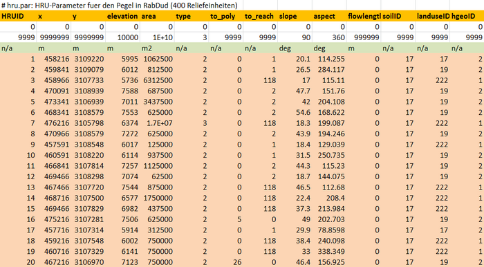
A sample HRU parameter file is provided below.

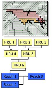
The HRU parameter file stores the spatial attributes of the catchment area where information about elevation, area, aspect, coordinates (x,y), land-use type (landuseID), hydrogeology(hgeoID) and soil(soilID) is stored for each HRU. The HRUs are topologically connected for lateral routing to simulate lateral water transport processes from an HRU to an HRU and were further connected to a nearby reach for reach routing. The column (to_poly) defines the HRU which passes water to the next HRU.

The connection between the HRU parameter file and other parameter files is solved inside former. For example, in the HRU parameter file, the HRU id 1 has all the necessary information as required in the table above, including the land-use, the soil and geology type which the HRU1 belongs to:

• Reach parameter file (*reach.par)

parameter	description
ID	channel part ID
length	length
to-reach	ID of the underlying channel part
slope	slope
rough	roughness value according to MANNING
width	width

The reach parameter file stores the information about stream characteristics as well as the relationship between stream networks to accomplish reach routing. The reach parameter file contains information on the structure of the flow topology by noting the ID for every reach into which it transfers. The reach parameter is produced along with the HRU delineation process and also comprises the information as required in the table above.

With respect to the figure of the HRU parameter file above, the HRU ID 1 contributes water directly to REACH ID 1 whereas HRU ID 16 contributes water to HRU ID 5 which then contributes to REACH ID 2. The interactions between the parameter files were solved by a relation between soil, land use and hydrogeological descriptors in the HRU parameter file and respective descriptors in the other parameter files.

[Important] The sample parameter files are provided in the workspace directory.

Meteorological input data

The J2000 hydrological model requires the following input data for the model initialization:

name	description	unit
ahum.dat	absolute humidity	g/cm3
orun.dat	measured flow passage at the runoff	m3/s
rain.dat	measured amount of precipitation	mm
rhum.dat	relative humidity	%
sunh.dat	sunshine duration	h
tmax.dat	maximum temperature	°C
tmean.dat	mean air temperature	°C
tmin.dat	minimum temperature	°C
wind.dat	wind speed	m/s

The J2000 modelling system uses Inverse Distance Weightings (IDW) with the elevation correction method for the regionalization of the input climate data. The detailed description of the regionalization approach is provided in:

[Regionalization approach of the J2000]

All the data as shown in the above figure might not be available in some catchments. Normally, temperature and precipitation data are commonly available. If there are only few stations (less than 3) for some parameters, the IDW does not work properly. In that case, the same input value is applied for the entire catchment. For some particular variables, for example, temperature, this approach would bring large amounts of errors/uncertainties. In such cases, the regionalization approach based on a lapse rate is suggested for temperature. The details of this approach are provided in Nepal, 2012.

The relative humidity, wind and sunshine hours are also not frequently available in some catchments. These values are used for the estimation of evapotranspiration while using the Penman-Monteith approach. The sunshine hours and wind speed can be assumed to be enough from one station, in case no other station data is available. In such cases, the same station value is applied for a whole catchment. The one station value for relative humidity also brings certain errors while calculating relative humidity using absolute humidity and temperature. In the J2000 modelling system, a direct regionalization of the relative humidity values is not recommended. The details are provided in the calculation of evapotranspiration sub-tutorial.

In case these data (rhum, sunh, wind) are not available the Pennmann-Monteith approach cannot be used. Rather a more empirical approach based on temperature such as Hargreaves, can be used.

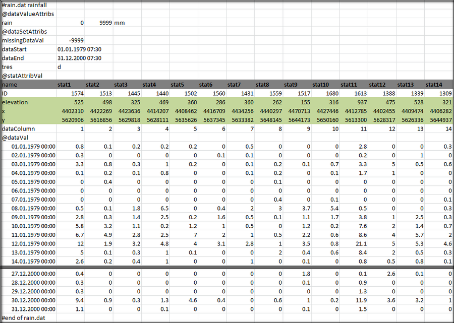
A sample of the Input data of the rainfall (rain.dat) file is provided below:

The input data must be saved with the extension .dat (example: rain.dat). The data in excel format can be saved as 'Text (tab delineated)(*.txt)' and changing the extension from *.txt to *.dat*. At the end of the each dataset, the data column must be ended by #end of data.dat. For more details, download the sample data file:

Each data file has the following structure (demonstrated here for the example "rainfall"):

line	description
#rain.dat rainfall
@dataValueAttribs
rain 0 9999 mm	name of the data series, smallest possible value, biggest possible value, unit
@dataSetAttribs
missingDataVal -9999	value to mark missing data values
dataStart 01.01.1979 7:30	date and time of the first data value
dataEnd 31.12.2000 7:30	date and time of the last data value
tres d	temporal resolution of the data (here: days)
@statAttribVal
name stat1 stat14	names of the rainfall stations
ID 1574... 1309	numeric id of the rainfall stations (ID)
elevation 525... 321	elevation station1... elevation station14
x 4402310... 4406282	easting station1... easting station14
y 5620906... 5644937	northing station1... northing station14
dataColumn 1... 14	number of the particular column in the data part
@dataVal	beginning of data part
01.01.1979 07:30 0.8... 0.3	date, time, value station1... station14
...
17.10.2000 07:30 0.1..0.1	date, time, value station1... station14
#end of rain.dat	end of data part

The sample files of input data can be downloaded from the workspace directory provided in here.

Workspace for input data

The input data of the J2000 hydrological model has to be provided in a specific folder considered as a 'workspace directory'. This directory contains all the input data required to run the model as well as the model output files. The workspace directory of 'Dudh Kosi model' is provided herewith with all the input dataset from 1987 to 1990 required to run the model. As explained earlier, the input data provided here are not from the observed stations. They are from some hypothetical stations derived from regioanlized data in addition to unsystematic random errors.

File:J2000 DudhKosi Tutorial.zip

Glacier module extension for the J2000 model

Important Note:

J2000Himalaya.zip contains a J2000Himalaya.jar file which is an extension of the glacier module to the standard J2000 hydrological model. Therefore, this jar file has to be copied in the lib folder (\Program Files\jams\lib) [if your basin has glaciers]. The lib folder already contains J2K.jar file when users download the JAMS software along with the test dataset of the Gelberg catchment. Users can also keep the J2000Himalaya.jar file in different locations, but the path has to be defined when the model is run first time by the following steps:

[JAMS laucher(or JAMS builder)-->>Edit-->>Edit perferences]. A new window 'JAMS preferences' will appear. Users need to locate the location of the *jar file by clicking + sign).

Folders and files

The workspace directory has three main folders: input, output and parameters. The input folder has all the required input data to run the model. The parameter folder has parameter files (hru.par, hgeo.par, landuse.par, soil.par and reach.par). The output folder contains output files of different variables after the model is successfully run. A sample workspace of test dataset is provided herewith which provides an idea of how to organize the workspace directory for the J2000 hydrological model.

Folder: input

The input folder has 12 xml files of all input data. Please copy and paste these files as they are the connector for the real input data which are located inside the folder 'local'.

subfolder: local

The folder the inside input folder contains the input data for eight variables (rain.dat, rhum.dat, sunh.dat, tmax.dat, tmean.dat, tmin.dat, wind.dat). ahum.dat is created when the model is run for the first time by using the existing data.

subfolder: gis

Some GIS layers can be put here to display the spatial distribution of some output variables (for example, the spatial distribution of precipitation in a catchment (2D and 3D). For this, users need to put the DEM file of a catchment (data format: *.asc). The resolution of the DEM should be similar to the input DEM for the HRU delineation process. Users need to copy the styles.sld file, which is required to display a map. Additionally, HRUs, streams and station data files (*.shp) can be put in a separate folder to display the variables in a map component. The names of these files and folders have to be defined in a model xml file [model xml file].

'subfolder: dump'

Create a folder with a name 'dump' which is used to dump temporary files.

Folder: output

The folder output has two xml files (HRULoop.xml and TimeLoop.xml) and a folder current. These *.xml file defines the variables for which the output is created. Similarly, the output data are put inside the current folder (file names: TimeLoop.dat and HRULoop.dat). The relevancy of these output data is discussed in the sub-tutorial 'Model output' below. [Subsection: Numerical display]

Folder: parameter

The folder contains parameter files (hgeo.par, hru.par, landuse.par, reach.par, soils.par). Please remember that these names should be same in the model xml file.

Folders: explorer and tmp

The other folder inside the workspace is the explorer and the tmp that is used to dump some temporary files generated while running the model.

Model xml file

The workspace directory also contains a model xml file. The model files can be read as *.xml or *.jams. These model files are provided in an example test dataset.

Definition of the Model xml file:

An example of few model xml files is provided herewith. Please unzip the file to use it.

File:J2k gehlberg.zip: This is a standard J2000 model xml file provided in the Gelberg test data. The Gelberg catchment in Germany has sufficient input data to use IDW method for regionalization

File:J2K DudhKosi SantoshPhD Tutorial 2.zip: This is a model xml file of the Dudh Kosi river basin in the Himalayan region. The region has only one temperature station. Therefore, Temperature lapse rate module is used for temperature regionalization.

File:J2k Hargreves.zip: This is a model xml file for data scarce region (temperature and precipitation only) and the potential evapotranspiration is calculated using the Hargreaves Salami method.

By applying different modules, the data requirement for the model is changed. In such condition, different modules are disable or removed in the xml file. For example, for Hargreaves Salami module , the wind, sunshine hour and relative humidity is not required. Therefore, the data reader and regionalization of these parameters are disabled in the Hargreaves xml. If users want to use Hargreaves Salami module, it is advised that users compare the xml file and data requirements with Dudh Kosi or Gelberg xml.

The model xml file contains the logical structure of the model framework and modules used in the model. It is organized in a systematic way that output from one module is supplied as input to the next one (example: snowmelt (output from the snow module is an input for the soil water module). This file also contains information about the display of different variables and outputs in the JAMS framework. The model xml can be viewed using the JAMS builder to understand the different component of a specific model.

Users can follow this tutorial to get familiar with the JAMS Builder. This tutorial is very important to understand different fuctions of JAMS builders. For example, how to upload an existing model, how to create a new model.

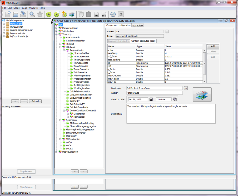
An example of the Dudh Kosi model is provided in the JAMS builder in the figure below.

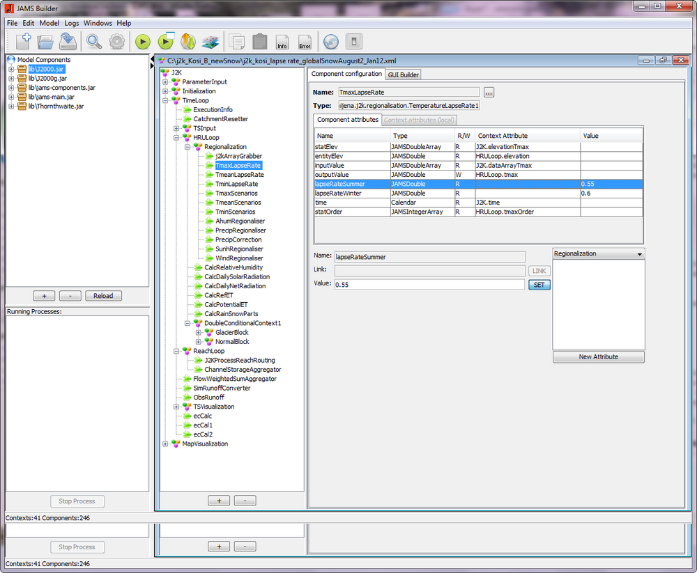
The left window shows the location of model source code files which are required to run a model. All the model source codes are inside the *.jar file. For the J2000 model, a J2000.jar file is used. The middle window provides information about the modules used in the model xml file of the Dudh Kosi model. These are provided in logical structure where the output of one module is provided as input to next. A detailed description of these different modules will be provided in the subsequent section. An example of the Maximum temperature regionalisation module (TmaxLapseRate) is shown in the JAMS builder below. The module uses single station temperature data to regionalize the maximum temperature in a catchment. By clicking the TmaxLapseRate in the middle column under Regionalization, the detailed information of the module is displayed in the right windows as shown in the figure below.

All the variables used in the modules are provided under the column 'Name' as shown in Figure above. The column 'Type' describes the characteristics of variables in terms of the information (data, quality) they store in these variables. The column 'R/W' determines their input and output nature. Such as 'statElev' is a elevation of a temperature station which is denoted by R. This means that the information is input to the module from a previous module and denoted by 'Read'. The 'W' denotes Write which is the new output value from this module. The calibration parameters, if any, are provided in the column 'Value'. This information can be changed from JAMS builder instantly. Upon clicking the variable, the information on 'attribute configuration' will be filled. This information can be changed. Please click on 'set' to save the information.

The model can be run from JAMS builder by clicking the button 'Run Model [1]' or 'Run Model from JAMS launcher[2]' as denoted by red box in the figure below. Clicking the box "1" will directly launch the model, whereas the box "2" will launch JAMS launcher. The latter will provide options to change the model parameters (such as parameter values, time period)etc.

A more detailed description of the model xml file in relation to different modules and variables used in the model source codes are described in Krause (2011). This document can be generated from the JAMS builder instantly. Click on the 'Model' from top banner and 'Generate Model Documentation'. The model documentation will be available in pdf format for download.

The model xml can also be viewed and edited using a text editor software (such as PSPad) as shown below for the 'Maximum Temperature Regionalization module'.

---

<component class="org.unijena.j2k.regionalisation.TemperatureLapseRate1" name="TmaxLapseRate">

• This line defines the location of the module TemperatureLapseRate1 in the model library file *J2000.jar.

<var name="lapseRateWinter" value="0.6"/>
<var name="lapseRateSummer" value="0.55"/>

• The value of lapseRateWinter and lapserateSummer is the calibration parameter which is a lapse rate of change in temperature per 100 meter.

<var attribute="elevation" context="HRULoop" name="entityElev"/>

• The attribute elevation defines the elevation of an HRU which is the input variable to the TemperatureLapseRate1 module. The model reads the elevation of each HRU from the HRU parameter file as explained earlier.

<var attribute="time" context="J2K" name="time"/>

• time defines the temporal resolution of the model (eg. daily)

<var attribute="tmax" context="HRULoop" name="outputValue"/>

• tmax is the maximum temperature as an output value from the module. It calculates a maximum temperature for each HRU using the input variables inside the module.

<var attribute="elevationTmax" context="J2K" name="statElev"/>

• elevationTmax is the input variable of elevation of maximum temperature station. The model read the elevation from the temperature station in an input file (e.g. tmax.dat).

<var attribute="dataArrayTmax" context="J2K" name="inputValue"/>

• dataArrayTmax is the input variable of maximum temperature on a particular date.

<var attribute="tmaxOrder" context="HRULoop" name="statOrder"/>

• tmaxOrder defines the order of the station in case more than 1 temperature station is available based on the distance of an HRU with the temperature station. In that case, the model recognizes the nearby station from the particular HRU.

The logical order of the variables used in the module is very important in the model xml file. For example, each input variable must be defined earlier before it is used. For example, the input variable 'dataArrayTmax' is defined earlier in a module called 'TmaxDataReader'. The module reads all the maximum temperature daily data in a format which the model can recognize. Similarly, the output variable 'tmax'(maximum temperature) is then used in a later section. For example: the tmax (maximum temperature) value of each HRU is used to calculate its snowmelt.

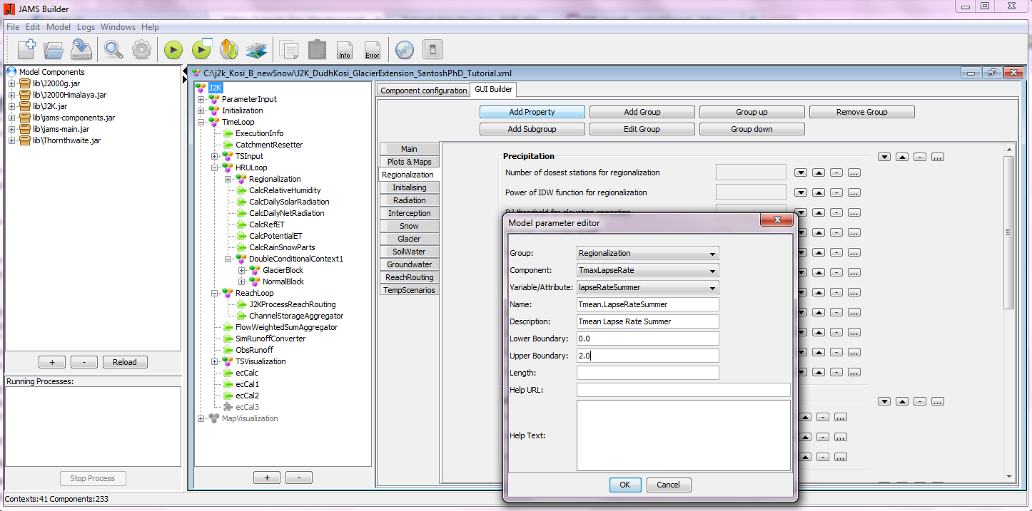
The calibration parameters can be displayed in the JAMS framework before running the model. For this, the GUI builder of the JAMS launcher can be used (Figure below). Here the example for the Temperature lapse rate has been shown. The temperature lapse rate can be kept under the group regionalization.

1. First click on the GUI builder and choose the group 'regionalization' and then click on 'add properties'. A new window 'Model parameter editor' will appear where the information of the model component can be changed.

2. For example, in the 'Component' class, choose TmaxLapseRate. In Variable/attribute, choose lapseRateSummer. Similarly, the name and description of the parameter also have to be filled, along with its lower and upper boundary of the parameter. Users can choose the calibration parameter in between the boundary range. They can also put extra information under Help Text to provide more detailed information about the parameter. When all the information is filled in, clicking "OK", will bring the parameter in the modelling framework. Likewise, in the next step, users can choose the 'lapseRateWinter' for TmaxLapseRate. This is due to the maximum temperature being regionalized with two different lapse rates for summer and winter and also fill in the other information as required as shown in the figure below:

The same process can be repeated with TmeanLapseRate and TminLapseRate for summer and winter periods.

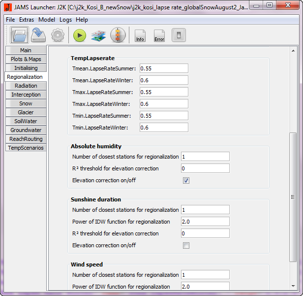
The figure below shows the calibration parameters for the lapse rate which are displayed in the JAMS framework. Users can change the value from the JAMS launcher before running the model.

Display model results and output

The xml file comprises components to display model results of certain variables. The model output results can be viewed in the JAMS window after running the model. The spatial distribution of certain output variables (such as precipitation, evapotranspiration) can be displayed at the end of the model run, including the 3D map. In addition, the model also provides the different efficiency results of statistical evaluation at the end of the model run.

The description of the output of model results are provided in the following sub-tutorial: [Output of model results]

Modules within the J2000 hydrological Model

This section describes the different modules within the J2000 hydrological model. The calibration parameters applicable to each module are also described with focus on their influence on streamflow. Following are the important modules in the J2000 hydrological model.

• Precipitation distribution module
• Interception module
• Snow module
• Glacier module
• Interception module
• Soil module
• Groundwater module
• Lateral routing
• Reach routing

Calculation of Evapotranspiration

The detailed description of calculation of evapotranspiration using the Pennmann-Monteith approach (Allen, 1998) is provided in this sub-tutorial.

[Calculation of evapotranspiration]

Precipitation distribution module

Calibration parameters

Parameters	Description	Global range	For the Dudh Kosi model
Trans	threshold temperature	0 to - 5	2
Trs	base temperature for snow and rain	-5 to +5	0

These parameters are considered as non-flexible parameters and not necessarily placed in the JAMS framework as tunable parameters.

In the J2000 modelling system, the precipitation is first distributed between rain and snow depending upon the air temperature. Two calibration parameters (Trans, and Trs) are used where Trs is base temperature and Trans is a temperature range (upper and lower boundary) above and below the base temperature. In order to determine the amount snow and rain, it is assumed that precipitation below a certain threshold temperatures results in total snow precipitation and exceeding a second threshold results in total rainfall as precipitation. In the range (Trans) between those threshold temperatures, mixed precipitation occurs.

Relevancy in modelling

Putting the Trs values below zero (e.g. -2) will bring more precipitation in the form of 'rain' than 'snow'.

The detailed description of this module along with the algorithm as defined in the model source code is provided in: [Precipitation distribution module]

Interception module

Calibration parameters

Parameters (units)	Description	Global range	For the Dudh Kosi model
α_rain (mm)	storage capacity (m²) of particular land cover for rain in mm	0 to +5	1.0
α_snow (mm)	storage capacity (m²) of particular land cover for snow in mm	0 to +5	1.28

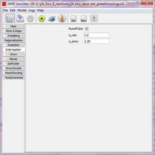
The calibration parameters of the interception module in the JAMS builder is provided in the figure below:

Interception is a process during which the precipitation is stored in leaves, and other open surfaces of vegetation. This process is identified as important components of a hydrological cycle that can affect the water balance components. Canopy and residue interception are considered losses to the system, as any rainfall intercepted by either of these components will subsequently be reduced by the evapotranspiration process. The interception module uses a simple storage approach according to Dickinson (1984), which calculates a maximum interception storage capacity based on the Leaf Area Index (LAI) of the particular type of land cover. The model gets the LAI information of different seasons from the land-cover parameter file. When the maximum storage is reached, the surplus is passed as throughfall to the soil module.

The parameters as shown in the figure above have a different value, depending on the type of the intercepted precipitation (rain or snow). It is because the maximum interception capacity of snow is noticeably higher than of liquid precipitation.

Relevancy in modelling

Keeping the high value of parameters (a_snow and a_rain) will store more water on leave surfaces which leads to higher evapotranspiration and less water available for next module (i.e. soil module) runoff and vice versa.

The detailed description of this module along with the algorithm as defined in the model source code is provided in: [Interception module]

Snow module

Calibration parameters

Parameters (units)	Description	Global range	For the Dudh Kosi model
snowCritDens (%)	Critical density of snowpack	0 to 1	0.381
snowColdContent	cold content of snowpack	0 to 1	0.0012
baseTemp (oC)	threshold temperature for snowmelt	-5 to 5	0
t_factor	melt factor by sensible heat	0 to 5	2.84
r_factor	melt factor by liquid precipitation	0 to 5	0.21
g_factor	melt factor by soil heat flow	0 to 5	3.73

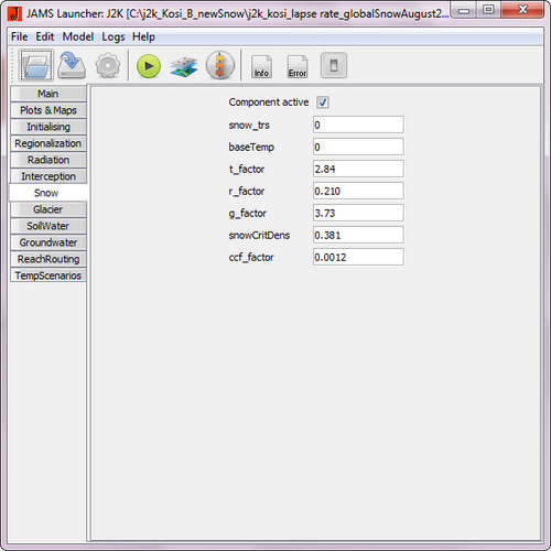
The calibration parameters of the snow module in the JAMS builder is provided in the figure below:

The J2000 snow module is carried out according to the method described in Knauf (1976) including some changes and extensions. The module estimates different state variables of the snow pack such as snow depth, snow density and snow water equivalent, which can be used for the process oriented multi-response validation. The module mainly describes the accumulation, melting and subsidence phases of a snow pack.

If the melt temperature exceeds the temperature limit value ( baseTemp), the snowmelt process begins. The snowColdContent parameter takes into account the cold content of the snow pack. The temperature of the snow pack has to be close to 0 to start the snowmelt process. Negative air temperatures are accumulated and decreased only by positive temperatures and to realize the snowmelt process.

The melt energy required for the calculation of potential snow melt is supplied in the form of sensible heat by air temperature (t_factor), energy input from precipitation as rain (r_factor) and input due to soil heat flow (g_factor). This potential melt rate is further modified according to slope and aspect of the HRU. The snow pack is able to store is liquid water (as supplied in the form of potential snow melt) in its pores up to a certain density limit (CritDens). This storage capacity is lost almost completely and irreversibly when reaching a certain critical density of the snowpack (i.e. amount of free water in relation to the total snow-water equivalent between 40% and 45%) according to (Bertle 1966; Herrmann 1976). The resulting snow snowmelt is supplied to the soil module.

Relevancy in modelling

baseTemp is a threshold temperature for snow melt. The melting only occurs if the air temperature is higher than baseTemp. Keeping the value high will make more snow to store and less snowmelt occurs and vice versa. This parameter is very important in case the basin has seasonal snow storage and melt. The best value can be found around the value 0.

snowCritDens is an important calibration parameter as this allows liquid water from snowpack to be melt when the critical density is higher than this value. This storage capability is lost nearly completely and irreversibly when a certain amount of liquid water proportionally to the total snow water equivalent (around 40%) is reached. Keeping this parameter value low will release the liquid water from snowpack quickly (as the critical density of snow is reached faster ) with less amount of snow and related depth. The high value of this parameter results more time to reach the critical density which will require more fresh snow to occur.

snowColdContent helps to reach the cold content of a snowpack close to zero so that the melting process start. Higher value will help to reach the cold content of a snowpack to zero faster than low value.

t_factor is one of the most important and sensitive parameters to produce melt runoff from a snowpack. The higher value will produce higher snowmelt and vice versa for low value. The higher t_factor value along with r_factor and g_factor will provide heat energy to melt the snowpack and produce runoff.

The detailed description of this module along with the algorithm as defined in the model source code is provided in: [Snow module]

Glacier module

Calibration parameters

Parameters (units)	Description	Global range	For the Dudh Kosi model
meltFactorIce	melt factor for Ice	0 to 5	2.5
tbase (oC)	threshold temperature for melt	-5 to 5	-1
debrisFactor	debris factor for ice melt	0 to 10	3
alphaIce	radiation melt factor for ice	0 to 5	0.2
kIce	melt factor by sensible heat	0 to 50	5
kSnow	melt factor by liquid precipitation	0 to 50	5
kRain	melt factor by soil heat flow	0 to 50	3

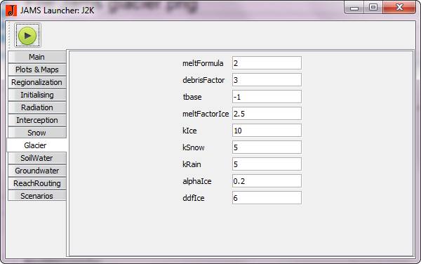
The calibration parameters of the glacier module in the JAMS builder is provided in the figure below. Users can choose the method to calculate the glacier icemelt between simple degree-day [1] factor and enhanced degree-day factor [2] in the 'melt formula'. The calibration parameter at the bottom 'ddfIce' is applicable for the simple degree day factor [1].

The seasonal or fresh snow in glacier areas are processed using the J2KProcessSnow as described in the Snow Module in the previous section. When snow storage is zero in the glacier HRU, the glacier ice melt process begins using the enhanced degree day factor. The energy for glacier ice melt is represented by the degree-day factor which is the general function of temperature and radiation (meltFactorIce and alphaIce). The melt rate is further adapted to slope and aspect of the specific HRU. The model also segregates the debris covered and non-debris covered glacier HRU by using the slope of HRUs. If the slope is higher than 30 degree, the glacier HRU is considered as non-debris covered glaciers. In the debris covered glacier HRU, the ice melt is further controlled by the calibration parameter debrisFactor. The outcome from the glacier area is snowmelt (from fresh snow), glacier ice melt and rain runoff (rain-on-glaciers). All these three melt runoff are routed through the glacier areas using three different routing for snow, ice and rain (kSnow, KIce and kRain). At the end, the glacier melt, which is the product of three different runoff (snowmelt, icemelt and rain runoff), are supplied to nearby reach as overland flow (RD1).

Relevancy in modelling:

meltFactorIce is one of the sensitive parameters of the glacier module. The higher value causes higher glacier ice melt and vice versa.

tbase is a threshold temperature for snow melt. The melting only occurs if the air temperature is higher than tbase. Keeping the value high will make more snow to store and less snowmelt occurs and vice versa. The best value can be found around the value 0.

debrisFactor controls the ice melt. The higher value (e.g. 4) means the icemelt is reduced by 40% in the debris covered glacier.

alphaIce bring the radiation factor for snowmelt. The higher value will cause higher glacier ice melt.

kIce, kSnow and kRain are routing coefficient. The lower values represents the short residential time of the potential melt runoff. It is assumed that the rain on glacier surface drains faster than snowmelt and icemelt.

The detailed description of the glacier module along with the algorithm as defined in the model source code is provided in Glacier Module

Soil water module

Calibration parameters

Parameters (units)	Description	Global range	For the Dudh Kosi model
soilMaxDPS (mm)	maximum depression storage	0 to 10	2
soilLinRed	linear reduction co-efficient for AET	-5 to 5	-1
soilMaxInfSummer (mm)	maximum infiltration in summer	0 to 200	60
soilMaxInfWinter (mm)	maximum infiltration in winter	0 to 200	75
soilMaxInfSnow (mm)	maximum infiltration in snow cover areas	0 to 200	40
soilImpGT80	infiltration for areas greater than 80% sealing	0 to 1	0.5
soilImpLT80	infiltration for areas lesser than 80% sealing	0 to 1	0.5
soilDistMPSLPS	MPS-LPS distribution coefficient	0 to 10	0.3
soilDiffMPSLPS	MPS-LPS diffusion coefficient	0 to 10	0.5
soilOutLPS	outflow coefficient for LPS	0 to 10	0.3
soilLatVertLPS	lateral vertical distribution coefficient	0 to 10	0.5
soilMaxPerc (mm)	maximum percolation rate to groundwater	0 to 100	10
soilConcRD1Flood	recession coefficient for flood event	0 to 10	1.3
soilConcRD1Floodthreshold	threshold value for soilConcRD1Flood	0 to 500	300
soilConcRD1	recession coefficient for overland flow	0 to 10	2.8
soilConcRD2	recession coefficient for Interflow	0 to 10	3

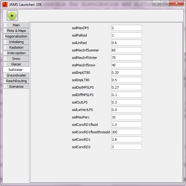
The calibration parameters of the soil water module in the JAMS builder is provided in the figure below:

The soil module is the most complex part of the J2000 hydrological model which reflects the central role of the soil zone as a regulation and distribution system. The input for the soil module is snowmelt and precipitation in the form of rain. The middle pore storage (MPS) and large pore storage (LPS) represents the water holding capacity of the soil. The water in the MPS represents the field capacity in which water is held against gravity but can be subtracted by an active tension eg. plant transpiration. The input to the soil module is first used to fill the MPS and LPS, which determines the current soil moisture. The soil moisture conditions influence the infiltration process. The infiltration capacity of the particular soil is calculated based the actual soil moisture. Besides this, there are three different infiltration parameters (soilMaxInfSummer, soilMaxInfWinter and soilMaxInfsnow) which controls the infiltration during summer, winter and snow cover. In case of the sealed areas, only certain amount of water on the surface is able to infiltrate which is controlled by two parameters (soilImpGT80 and soilImpLT80). The water which is not able to infiltrate is stored at the land surface, as depression storage, up to a certain amount as defined in calibration parameter (soilMaxDPS) and any surplus is treated as overland flow (RD1). The infiltrated water is then distributed between the MPS and LPS which is controlled by two calibration parameters (soilDistMPSLPS and soilDiffMPSLPS). The water available in MPS can be reduced by evapotranspiration for which the root depth of the respective land cover in the soil is important. The water is the LPS is distributed between the lateral and vertical components (soilLatVertLPS). The lateral flow is responsible for producing interflow from the unsaturated zone (RD2) which can be controlled by soilOutLPS. The vertical flow (percolation) is supplied to groundwater zone (saturated zone) for which the rate of percolation is controlled by soilMaxPerc. The surplus is supplied to the LPS to release as overland flow (RD2). The overland flow and Interflow 2 are controlled by retention coefficient (soilConcRD1 and soilConcRD2).

In the case of overland flow, the retention time period may be different during high flow periods due to non-linear behavior of a catchment. For this, new parameters are introduced to represent the non-linear behavior during the monsoon season of the Himalayan region. Therefore, a new parameter (soilConcRD1Flood), as a recession co-efficient for overland flow during high flood peak period, when the volume of overland flow crosses the threshold soilConcRD1Floodthreshold defined as a calibration parameter.

Relevancy in modelling

soilMaxDPS influences the water stored in depression areas. The higher value of this parameter causes higher amount of water to be stored as depression storage and less water to be available for overland flow.

soilLinRed reduces the amount of evapotranspiration rate. The lower value will reduce the evapotranspiration at a lower rate.

soilMaxInfSummer, soilMaxInfWinter, and soilMaxInfSnow influence the maximum infiltration rate into the saturated (soil water) and unsaturated (groundwater) zone. The lower value of these parameters allow only a part of rainfall and snowmelt to enter into the unsaturated zone (The value 20 means that only 20 mm rainfall and snowmelt is allowed to go through the soil water module per time step). In such cases, overland flow would be higher as the most of the input drains as surface runoff. It is considered that the soilMaxInfSummer is slightly lower than winter because the soil is more saturated during the rainy-summer period. The soilMaxInfSnow is considered lowest among the three because of the frozen soil condition in the snow-occurring environment.

The parameter soilImpGT80 is activated if the land cover impermeability is high as defined in the permeability of the land cover (sealedgrade) (such as urbanized areas) in the land-cover parameter file. The values in the sealedgrade act as a threshold for activation of the parameters soilImpGT80 or soilImpLT80. The lower value of these parameters indicates that the lower amount of inflow will be able to infiltrate and rest flow as overland flow.

soilDistMPSLPS and soilDiffMPSLPS are mainly responsible for distribution and diffusion of water between the MPS and LPS. They are less sensitive parameters and have minor role in interflow. The lower value of these parameters will allocate slightly less inflow to the MPS.

soilOutLPS influences the Interflow 2 (RD2) component. The lower value will allocate more water to be outflowed from LPS and thereby increasing the RD2 component.

soilLatVertLPS is one of the very sensitive parameters in the soil water module. It distributes the inflow (after the infiltration) between vertical (interflow 1) and percolation. The higher value will allocate higher amount of inflow to the Interflow 2 (and less inflow  to be percolated to the groundwater). The higher value will increase in Interflow 2 component and at the same time, the groundwater contribution (RG1 and RG2) will be reduced.

soilMaxPerc controls the percolation rate to the groundwater per time step. The higher (eg. 20) value indicates that maximum 20 mm equivalent water is allowed to go to the groundwater. The higher value will increase the groundwater contribution (RG1 and RG2) and at the same time decrease RD2 component at a higher magnitude. This also decrease the RD1 but to a lesser extent.

soilConcRD1 and soilConcRD2 are recession coefficient for overland flow (RD1) and Interflow 1 (RD2) and are one of the sensitive parameters in the module. The value represents the retention time (per time step) for overland flow. The higher value indicates that the retention period is high and therefore, less water is flowed as overland flow. Principally, the retention period for RD1 should be less than the RD2.

soilConcRD1Flood parameter is implemented in the standard J2000 hydrological model to replicate the runoff behavior especially during the high flood period in the monsoon dominated Himalayan region. This parameter is only activated when the input for overland flow crosses the parameter soilConcRD1FloodThreshold defined by users. In principal, the value of soilConcRD1Flood should be less than soilConcRD1 as the retention time of the overland flow is less during the high flood time.

The detailed description of the soil water module along with the algorithm as defined in the model source code is provided in Soil Water Module.

Groundwater module

Calibration parameters

Parameters (units)	Description	Global range	For the Dudh Kosi model
gwRG1RG2dist	RG1-RG2 distribution coefficient	0 to 10	2.1
gwRG1Fact	adaptation for RG1 flow	0 to 10	0.3
gwRG2Fact	adaptation for RG2 flow	0 to 10	0.5
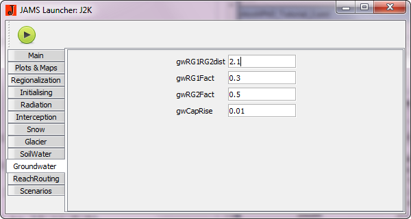
gwCapRise	capillary rise coefficient	0 to 10	0.01

The calibration parameters of the groundwater module in the JAMS builder is provided in the figure below:

The groundwater module receives input from unsaturated soil zone (soil water module) in a two storage compartment of a ground water zone i.e. upper groundwater zone (RG1) and lower grounwater zone (RG2). The input is then between these two zones in which the distribution of input is carried out by the calibration parameter gwRG1RG2dist. The water discharge from the upper and lower storage areas (RG1 and RG2) is carried out according to the current storage amount in the form of a linear function, using the storage retention co-efficient for two storages gwRG1Fact and gwRG2Fact. There is also a possibility that the water from groundwater is transfered soil water zone through capillary rise with the parameter gwCapRise.

Relevancy in modelling

gwRG1RG2dist distributes input water to RG1 and RG2. The higher value of this parameter increase the proportion of input water to the RG2 zone.

gwRG1Fact and gwRG2Fact influences the outflow from RG1 and RG2 storage. The parameter values represent the retention time in those stroage. The higher value will lead to less outflow and more water remains in the storage.

gwCapRise influece the distribution of water between soil water and ground water module. The higher value will flow a higher amount of water from groundwater to soil water zone.

The detailed description of the groundwater module along with the algorithm as defined in the model source code is provided in Groundwater Module.

Routing module

Calibration parameters

Parameters	Description	Global range	For the Dudh Kosi model
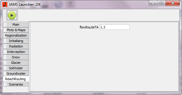
flowRouteTA	calibration parameter for adapting velocity of flow waves	0 to 10	1.3

The calibration parameters of the reach routing module in the JAMS builder is provided in the figure below:

The J2000 hydrological model has two routing components. The lateral routing serves to simulate lateral flow processes in the catchment area from one model entity (HRU) to the next until the water is finally reaches to a reach. The reach routing describes flow processes in a stream channel by using the commonly applied kinematic wave approach and the calculation of velocity according to Manning and Strickler (Krause, 2001).

Relevancy in modelling

flowRouteTA influences the run time of runoff waves in the stream channel. The higher value increases the velocity of runoff waves and more water flows from the channel.

The detailed description of the routing module along with the algorithm as defined in the model source code is provided in Routing module.

Model calibration

In order to apply hydrological models successfully it is necessary to define model parameters accurately. A direct measurement of the parameters is mostly not possible, too expensive or there is no clear physical relation. For those reasons the parameters are adjusted in a trial and error process in so far that the simulated factors (e.g. runoff) correspond best to the values measured. This task can be time-consuming and difficult if the corresponding model is complex or has a large number of parameters.

The J2000 model provides platform for offline and online calibration process. The offline calibration is carried within the JAMS framework, whereas in the online calibration, the model files and necessary parameters are defined in the web based calibration tools called 'OPTAS'. Then, the calibration is carried out in the server of the University and results can be downloaded. The latter is efficient and less time consuming as the calculation are carried out in server without making the local computers busy.

The detailed information about the model calirbation are provided in Model calibration

The model parameters, the specific values including the parameter ranges of the Dudh Kosi model are explained earlier in each modules. These parameter values were defined by combination of 'trail-and-error' and using automatic or numerical parameter optimization methods. The description of these methods and process are described in Nepal (2012).

Setting up a new model

To set up the J2000 hydrological model for a new catchment needs two important steps. First, prepare the model parameter files and input data as explained in the previous sections. Second, set up a new model xml file which controls the input and output variables based on the input data. The model xml file is different in different model application, as driven by input data and different modules used to calculate hydrological processes. (for example: the data requirement for estimating potential evapotranspiration using Hargreave-Salami method is different than the Penmann-Monteith, and therefore, the model xml set up is also different.

It is recommended to use the existing model xml files as a basis to set up a new model which has been provided in earlier sections. If the catchment has glaciers, users need to use the model xml of the Dudh Kosi river basin. Other than glaciers, users can use the model xml file of the Gelberg catchment which is provided while downloading JAMS software as a test dataset. These model xml files can be further changed based on the data requirements and preferences of the users.

In addition, users need to take into account few specific characteristics of the new catchment in the model xml file.

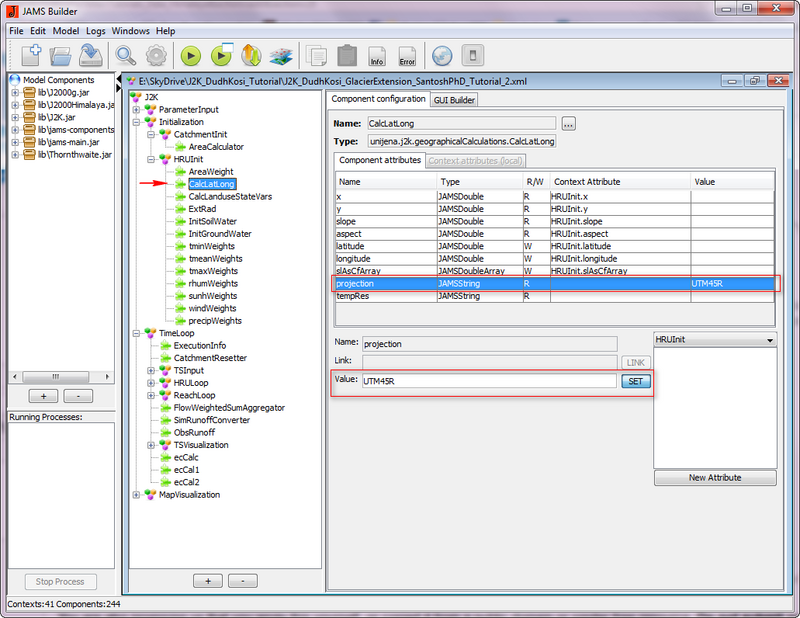
1. The geographical coordinates of the study area in UTM has to be defined in 'CalcLatLong' component to estimate 'slope aspect correction factor' as shown in figure below.

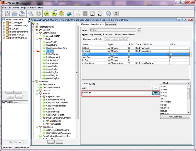
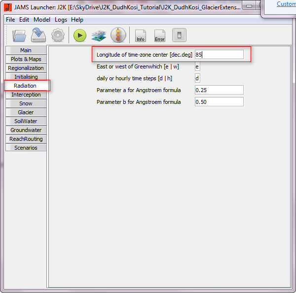
2. The geographical coordinates of the study area has to be defined in 'Calculate extra terrestrial radiation(ExtRad)' component based on the latitude and longitude. This can be done by editing the information in JAMS builder as shown in the figure below:

Alternatively, the information can be changed directly from JAMS laucher.

Please do not forget to save the new information.

3. The J2000 modelling sytem is quite flexible in terms of using different components based on the data availability. In the test dataset provided in this tutorial, for temperature regionalization, the data from one station is used and regionalized by summer and winter using lapse rate. But, if users have more than 3 stations data, they can use Inverse Distance Weightings (IDW) also. For this, users need to replace the IDW regionalization module with the Lapse rate module. Both these modules are provided in two different xmls above.

Similarly, to estimate evapotranspiration using Penmann Monteith, users need many data such as: relative humidity, wind and sunshine hour. These data might not be available in many areas. In such cases, alternative module for evapotranspiration named 'Hargreaves' can be used in the model.

Users need to be careful that while changing modules in standard xml provided here (Dudh Kosi and Gelberg), the data requirements also change. Because of this some modules might not be required in new model set up. For example, if Hargreves method is used, the data reader component and regionalization component for relative humidity, wind and sunshine hour is not required. In such cases, these modules has to be deactivated.

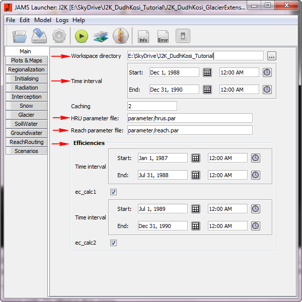
4. The location of workspace directory and some data file has to be defined after launching the model xml file as shown in the figure below.

The model xml file is opend using JAMS builder or JAMS launcher [File-->Load Model].

Workspace directory: The location of workspace directory in the local machine.

Time Interval: The time period in which the model is run.

Parameter file: The location of HRU and Reach parameter file.

Efficiency: Users can give the different time period for efficiency estimation.

Discussion Forum

It is likely that while while using the model and tutorial, users might encoutner probelms and error messages. In such cases, users are advised to contact the ILMS model discussion forum from where the model users and developer communities can be reached.

Integrated Land Management System (ILMS) discussion forum:

http://ilms.uni-jena.de/ilms/board/index.php?sid=f545b1932d03a6781393eea0fed040e3

The ILMS discussion forum is designed to discuss the various components of ILMS software. For the ILMS Model, the following forum is allocated:

http://ilms.uni-jena.de/ilms/board/viewforum.php?f=6

Users can also register in the ILMS forum Register here