Set Evaluation criteria
(→prozentualer Volumenfehler (PBIAS)) |
(→Nash-Sutcliffe-Effizienz(E2)) |
||
| Line 10: | Line 10: | ||
==Nash-Sutcliffe-Effizienz(E2)== | ==Nash-Sutcliffe-Effizienz(E2)== | ||
| − | + | The Nash-Sutcliffe Effizienz E2 (Nash und Sutcliffe, 1970) | |
<math> E_2 (\theta) = 1 - { \sum_{i=1}^r (o_{t_i} -y_{t_i})^2 \over \sum\limits^{r}_{t=1} ( o_{t_i}- \overline o )^2 } \quad \mathrm { mit} \quad \overline o = \frac {1}{r} \sum\limits^{r}_{t=1} o_{t_i} </math> | <math> E_2 (\theta) = 1 - { \sum_{i=1}^r (o_{t_i} -y_{t_i})^2 \over \sum\limits^{r}_{t=1} ( o_{t_i}- \overline o )^2 } \quad \mathrm { mit} \quad \overline o = \frac {1}{r} \sum\limits^{r}_{t=1} o_{t_i} </math> | ||
TODO:Formel einfügen | TODO:Formel einfügen | ||
| − | + | ||
| − | + | is definated as one monus the sum of absolute quadratic aberration, that will be normalized with the variance of observation in the viewed period. The range of the Nash-Sutcliffe efficience reaches from minus till plus one. It has its maxiums if both timelines are in conform. An negativ value means, that the modell rated the observation less than the middlevalue of observation. E2 is used very often, but has some disadvantages. Aberrances are quadratic calculated, therefore are higher drainvalues stronger judged than lower drainvalues. But as an result it is perfectly used for evaluation of highwaterperiods and drainpikes (Legates and McCabe Jr, 1999). Schaefli and Gupta (2007) made a point, that E2 depends from the statistical spread of the timelines and therefore is only areaspecificaly. Thats why the Nash-Sutcliffe efficience can only be used restricted to compare different areas. | |
| − | + | ||
| − | + | ||
| − | + | ||
| − | + | ||
| − | + | ||
| − | + | ||
| − | + | ||
| − | + | ||
==Die modifizierte Nash-Sutcliffe Effizienz E1== | ==Die modifizierte Nash-Sutcliffe Effizienz E1== | ||
Revision as of 15:34, 9 April 2014
It is necessary to have evaluation criteria, to judge the efficiency of an simulation. Evaluation Criteria quantify the similarity of two timelines. Evaluationcriteria are used to check the quality of an simulation. Although they quantify the simularity of two timelines. That makes it an objective measure instrument for variance of a timeline when observated and on the other hand enable to make an evaluated comparisson of errorfunctions between multiple timelines with the focus on observation. It is an goal of automated calibriation to change modellparameters in that way, that the simularity of an simulated timeline to an observated timeline, get maximized. For this process are errorfunctions essential. There exists countless measures, to evaluate the modell performance, that execl through there individual pro and contras. Usually used measures are:
Contents |
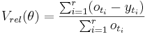
prozentualer Volumenfehler (PBIAS)
Measures the relative error between the simulated and the observated timeline. This measure shows, if the simulation follows a systematically over or unter rating.
Nash-Sutcliffe-Effizienz(E2)
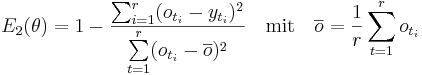
The Nash-Sutcliffe Effizienz E2 (Nash und Sutcliffe, 1970)
TODO:Formel einfügen
is definated as one monus the sum of absolute quadratic aberration, that will be normalized with the variance of observation in the viewed period. The range of the Nash-Sutcliffe efficience reaches from minus till plus one. It has its maxiums if both timelines are in conform. An negativ value means, that the modell rated the observation less than the middlevalue of observation. E2 is used very often, but has some disadvantages. Aberrances are quadratic calculated, therefore are higher drainvalues stronger judged than lower drainvalues. But as an result it is perfectly used for evaluation of highwaterperiods and drainpikes (Legates and McCabe Jr, 1999). Schaefli and Gupta (2007) made a point, that E2 depends from the statistical spread of the timelines and therefore is only areaspecificaly. Thats why the Nash-Sutcliffe efficience can only be used restricted to compare different areas.
Die modifizierte Nash-Sutcliffe Effizienz E1
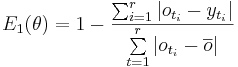
besitzt ähnliche Eigenschaften wie die gewöhnliche Nash-Sutcliffe Effizienz. Im Unterschied zu dieser werden die Abweichungen durch die gewöhnliche Betragsfunktion quantifiziert, so dass eine überproportionale Gewichtung der Abflussspitzen verhindert wird. Daher liefert diese Fehlerfunktion eine ausgewogenere Bewertung der Simulation (Krause et al., 2005).
logarithmierte Nash-Sutcliffe-Effizienz (logE2)
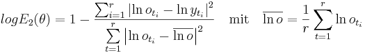
nimmt eine logarithmische Transformation der Werte vor, so dass hohe Werte (z. B. Abflussspitzen) gegenüber niedrigen Werten stärker abgeflacht werden. Dadurch wird die Gewichtung der niedrigen Abflüsse erhöht (Krause und Flügel, 2005).
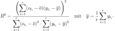
Bestimmtheitsmaß
Das Bestimmtheitsmaß R2 misst die Stärke des linearen Zusammenhangs zwischen beobachteter und simulierter Zeitreihe. Der Wertebereich dieses Maßes beträgt 0 bis 1. Nimmt dieses Maß den Wert 1,0 an, besteht ein perfekter linearer Zusammenhang zwischen der beobachteten und simulierten Zeitreihe. Im entgegengesetzten Fall (R2 = 0) lässt sich gar kein linearer Zusammenhang feststellen. Das Bestimmtheitsmaß beurteilt also nicht, ob zwei Zeitreihen quantitativ übereinstimmen, sondern nur ob sich ihre Dynamik ähnelt. Somit sollte die Bewertung von Hydrographen nicht allein mit diesem Maß durchgeführt werden (Krause et al., 2005). Das Bestimmtheitsmaß ist definiert als Quadrat des empirischen Korrelationskoeffizienten beider Zeitreihen:
Set evaluation criteria with the aid of JAMS Model Builder
You can find this option in the tab Configure Efficiencies. Now you should see the following window:

Now you can set , depending on your requirements of your callibration, criteria. As an example we show you here an minimal configuration :
1. step: Click on the button "+" , to create a new criteria.
2. step: Specifiy your attributs, that you want to compare. Both attributs must be set in the same contextcomponent. First chose from the drop-down-list the needed context, second the measured/observed and simulated attribut.
3. step: Chose an attribut, which represents the aktuell timestep of the simulation. Often, it should be "TimeLoop.time".
You should see a similar window like this:

4. step: click on OK to integrate the evaluation criteria to your model.