Módulos do J2000 em detalhes
m (→Módulo de neve) |
m (→Glacier module) |
||
| Linha 181: | Linha 181: | ||
Nos intervalos de tempo seguintes, a densidade da camada de neve mantém a densidade limiar crítica, até que a mesma seja descongelada ou inicie a acumulação devido à queda de neve recorrente. | Nos intervalos de tempo seguintes, a densidade da camada de neve mantém a densidade limiar crítica, até que a mesma seja descongelada ou inicie a acumulação devido à queda de neve recorrente. | ||
| − | = | + | = Módulo de geleira = |
| − | + | O módulo de geleira foi desenvolvido e adaptado como uma parte da pesquisa de doutorado (Nepal, 2012) realizado sobre a bacia hidrográfica do Kosi Dudh. As informações fornecidas aqui são tomadas a partir deste estudo. | |
| + | |||
| + | O módulo geleira está integrado no modelo hidrológico J2000 padrão, como parte desse estudo. Ele é tratado como um módulo separado dentro do J2000 em que o escoamento do degelo tanto da neve quanto do gelo (SIM) é calculada e resultado é passado diretamente a um rio como escoamento superficial (RD1). A abordagem sugerida por Hock (1999) foi implementada no modelo J2000 e ainda adaptada para a o cálculo do degelo. Esta abordagem considera o degelo utilizando um fator de dia-grau. A partir deste estudo, a inclinação, o aspecto e o fator de coberturas de detritos são ainda incluídos no modelo para o escoamento de degelo. O derretimento da neve na área glacial é calculada da mesma maneira como descrito anteriormente. O fluxo de calor do mesmo solo (parâmetro de calibração: g_factor) é proposto para o degelo nas zonas glaciais, já que a maioria das geleiras ficam cobertas por detritos e se comportam semelhante ao solo. | ||
| − | |||
| − | + | A área de geleira é fornecida como uma camada GIS que fornece uma ID exclusiva do uso da terra para as geleiras durante a delimitação da HRU. Todos os processos que ocorrem na geleira são tratados separadamente com base nessa identificação única. Primeiro a neve sazonal ocorre no topo da geleira (ou HRU de geleira). O modelo primeiro trata a neve, tal como descrito no “módulo de neve”, e produz o seu escoamento. A fim de se certificar de que o degelo ocorre, duas condições têm de ser preenchidas. Primeiro, a cobertura de neve inteira de uma HRU de geleira tem que derreter (ou seja o armazenamento deve ser zero). Em segundo lugar, a temperatura de base (''tbase''), tal como definida pelos utilizadores, tem de ser inferior a ''meltTemp''. Só nestas condições, o material fundido de gelo ocorre como um progresso de modelo. | |
Revisão das 19h56min de 26 de Fevereiro de 2013
Este tutorial descreve os processos importantes e algorítimos de diferentes módulos dentro do modelo hidrológico J2000 em detalhes:
Índice |
Módulo de distribuição de precipitação
- Parâmetros de calibração
| Parâmetro | Descrição | Variação global | Para o modelo Dudh Kosi |
|---|---|---|---|
| Trans | temperatura limiar | 0 + 5 | 2 |
| Trs | temperatura base para a neve e chuva | -5 +5 | 0 |
No sistema de modelagem J2000, a precipitação é primeiramente distribuída entre chuva e neve, dependendo da temperatura do ar. Dois parâmetros de calibração (trans e trs) são utilizados, sendo que trs é a temperatura base e trans é uma gama de temperatura (limite superior e inferior), acima e abaixo da temperatura base. A fim de determinar a quantidade de neve e chuva, presume-se que a precipitação abaixo de certas temperaturas limite resulta em precipitação totalmente de neve e acima de um segundo limite em precipitação totalmente em estado líquido. No intervalo (trans) entre as referidas temperaturas limite, a precipitação ocorre em forma mista. Entre esses limites, misturas de chuva e neve com percentuais variáveis para cada componente são calculadas. A quantidade de neve real (P (s)) da precipitação diária sujeita à temperatura do ar é calculada de acordo com:
![Ps = \frac{TRS + Trans - T}{2 \cdot Trans} \, \, \, \mathrm{[mm]}](/ilmswiki/pt/uploads/math/c/d/7/cd7e17fe47123cdcb7cf42c96cb2a604.png)
A quantidade diária de neve (Ps) ou a quantidade de chuva (Pr)são calculadas de acordo com:
![Ps = Precipitation \cdot Ps \,\,\, \mathrm{[mm]}](/ilmswiki/pt/uploads/math/6/c/f/6cf5aac907eba28aee593f2636d71204.png)
![Pr = Precipitation \cdot (1- Ps) \,\,\, \mathrm{[mm]}](/ilmswiki/pt/uploads/math/e/4/f/e4fca774452d67634b42a5ad62e02708.png)
Estes parâmetros são considerados como parâmetros não-flexíveis e não são necessariamente colocados no âmbito do JAMS como parâmetros ajustáveis.
- Relevâncias na modelagem
Configurar os valores trs abaixo de zero (por exemplo, 2) vai trazer mais precipitação sob a forma de "chuva" do que de "neve".
Módulo de interceptação
A interceptação é um processo durante o qual a precipitação é armazenada em folhas e outras superfícies abertas da vegetação. Durante a precipitação, ocorre a interceptação pelo dossel da plantas e de camada de resíduos. Este processo é identificado como componente importante de um ciclo hidrológico que pode afetar os componentes do balanço hídrico. A interceptação de copas e de resíduos é considerada uma perda para o sistema, já que qualquer chuva interceptada por qualquer um destes componentes subsequentemente evaporará (Kozak et al. 2007). O módulo de interceptação no sistema de modelagem J2000 serve como cálculo do volume de precipitação a partir da precipitação observada no contexto das coberturas vegetais particulares e do seu desenvolvimento no ciclo anual. A precipitação observada é reduzida pela parte interceptada para calcular-se o volume de precipitação. Assim a precipitação líquida apenas ocorre quando a capacidade máxima de armazenamento de interceptação da vegetação é atingida. O excedente é então repassado como precipitação interceptada para o próximo módulo. O módulo de interceptação utiliza uma abordagem simples de armazenamento de acordo com Dickinson (1984), que calcula a capacidade máxima de armazenamento de interceptação com base no Índice de Área Foliar (LAI), do tipo específico de cobertura do solo. O esvaziamento do armazenamento de interceptação é feito exclusivamente por evapotranspiração. A capacidade máxima de interceptação (Intmax) é calculada de acordo com a seguinte fórmula:
![Int_{max} = \alpha \cdot{LAI} \, \, \, \mathrm{[mm]}](/ilmswiki/pt/uploads/math/5/0/7/507166e6a6e240f947fac235bcc1a272.png)
com
α ... capacidade de armazenamento por m² de área foliar em relação ao tipo de precipitação [mm]
LAI ... LAI da classe de uso da terra especial previsto no arquivo de parâmetros do uso da terra [-]
O parâmetro “a” tem um valor diferente, dependendo do tipo da precipitação interceptada (chuva ou neve), visto que a capacidade máxima de interceptação da neve é sensivelmente mais elevada do que a precipitação em estado líquido. O LAI para os tipos de vegetação individuais é fornecido no arquivo de parâmetros de uso da terra ao longo do ano. Porque o LAI muda de acordo com as estações do ano, quatro tipos diferentes de LAI para quatro estações diferentes para cada tipo de vegetação são propostas no arquivo de parâmetro do uso da terra. O valor do LAI pode ser determinado por medição direta de folhas, literatura e conhecimento especializado.
Módulo de neve
- Parâmetros de calibração
| Parâmetro | Descrição | Variação global | Para modelo Dudh Kosi |
|---|---|---|---|
| snowCritDens | Densidade crítica de neve | 0 to 1 | 0.381 |
| snowColdContent | conteúdo de frio do bloco de neve | 0 to 1 | 0.0012 |
| baseTemp | temperatura de limite para fusão da neve | -5 to 5 | 0 |
| t_factor | fator de fusão pelo calor sensível | 0 to 5 | 2.84 |
| r_factor | fator de fusão pela precipitação líquida | 0 to 5 | 0.21 |
| g_factor | fator de fusão em pelo pelo fluxo de calor no solo | 0 to 5 | 3.73 |
Estes parâmetros são fornecidos em negrito e itálico na descrição abaixo:
O módulo de neve calcula as diferentes fases de acumulação de neve, metamorfose e neve derretida. O módulo mais complexo é adaptado no modelo de Knauf (1980). O módulo de neve leva em conta as mudanças de estado do bloco de neve durante a sua existência, especialmente suas mudanças de densidade devido ao degelo e a subsidência. Este processo é importante porque o bloco de neve pode armazenar água livre, como uma esponja, até atingir uma densidade de certo limite e só então uma descarga súbita de água ocorre. Para o modelo, capacidades diferentes de água da camada de neve são considerados: o equivalente real da água da neve (SWEdry) que corresponde à quantidade de água que realmente congelou e o equivalente total de água da neve (SWEtotal) que, além disso, considera a água em estado líquido armazenada no bloco de neve. A subsidência do bloco da neve, que resulta da água líquida através da fusão à superfície ou a partir da precipitação de chuva, é calculada de acordo com subsidência empírica (esquema de compactação da neve) por Bertle (1966).
A camada de neve e as suas condições estão descritas no modelo de acordo com os seguintes parâmetros: profundidade da neve (SD) [mm], a densidade da neve seca (dryDens)} [em g/cm³] como o quociente do teor total de água e da profundidade da neve.
Se houver uma temperatura do ar mínima, média e máxima para um determinado período de tempo (dados diários), o módulo calcula a acumulação separada ou temperaturas de fusão. A acumulação e fusão pode ocorrer dentro de um intervalo de tempo. As temperaturas de fusão e de acumulação (Tacc e Tmelt) podem ser calculadas de acordo com:
![T_{acc} = \frac{T_{min} + T_{avg}}{2} \,\,\,\,\,\,[^oC]](/ilmswiki/pt/uploads/math/3/d/3/3d3b5dd5170f4aeafe011df62d486968.png)
![T_{melt} = \frac{T_{max} + T_{avg}}{2} \,\,\,\,\,\,[^oC]](/ilmswiki/pt/uploads/math/c/3/a/c3a7020f5ca4f4668514ac77df26f8c7.png)
Fase de acumulação:
O módulo de neve simula a acumulação e a compactação da camada de neve causada pelo degelo ou chuva na precipitação de neve.
As circunstâncias térmicas sob a cobertura de neve são levadas em consideração juntamente com o teor de frio dessa cobertura em conexão com o degelo. Na temperatura abaixo do ponto de congelamento, o bloco de neve arrefece significativamente. Já que a água derretida congela imediatamente devido a circunstâncias isotérmicas negativas sob a cobertura de neve, não ocorre escoamento. O teor de frio tem de atingir o valor zero, de modo que o processo de degelo comece novamente. Consequentemente, as temperaturas negativas elevam o teor de frio enquanto que a temperatura positiva reduz-lo. O cálculo do armazenamento de conteúdo de frio resulta do produto da temperatura do ar por um parâmetro de calibração (coldContFact).
![CC = coldContFact \cdot T \,\,\,\,\,\,[mm]](/ilmswiki/pt/uploads/math/9/0/3/9035a165c2199ecd748ab631cf35b9fc.png)
Ao fazê-lo, temperaturas negativas do ar são acumuladas e diminudídas apenas por temperaturas positivas e pelas potenciais taxas resultantes de fusão. Só quando o teor de frio tiver atingido um valor de 0, ocorre o derretimento da neve.
Se a temperatura do ar for inferior a -15 ° C, pressupõe-se que a densidade da neve nova seja 0,02875.
A mudança de profundidade da neve (SD δ) resultante da precipitação da neve é calculada de acordo com seguinte premissa: a acumulação de neve ocorre no modelo se a precipitação cair sob a forma sólida (NewsNow> 0). Portanto, a densidade de neve nova é determinada sujeita a temperatura do ar. O cálculo é realizado de acordo com (Kuchment 1983, e Vehvilaeinen 1992), se a temperatura do ar for superior a -15 oC.
![newSnowDens = 0.13 + 0.0135 \cdot T_{acc} + 0.000045 \cdot T^{2}_{acc}\,\,\,\, [g/cm^3]](/ilmswiki/pt/uploads/math/7/0/8/708654912c93e6dbe77016e58c2bcc6f.png)
Se a temperatura do ar for inferior a -15 ° C, pressupõe-se que a densidade da neve nova seja 0,02875.
A mudança de profundidade da neve (SD δ) resultante de sua precipitação e é calculada da seguinte forma:
![δ SD = \frac{netSnow}{newSnowDens} \,\,\,\,\,\,[mm]](/ilmswiki/pt/uploads/math/3/c/1/3c1eba867cecfba876f54c0ad03f1a3b.png)
O equivalente de água da neve do dia anterior (\textit{SWEdry}) aumenta o valor de precipitação de neve de acordo com:
![SWEdry_{{t}} = SWEdry_{{t-1}} + netSnow \,\,\,\,\,\,[mm]](/ilmswiki/pt/uploads/math/d/c/f/dcf615c268a629e1153e30e9b4ad6fe8.png)
O equivalente de água da neve seca e o equivalente total de água da neve são aumentados pelo mesmo valor. Se o evento de precipitação envolvido precipitação mista (chuva/neve), a quantidade de chuva é atribuída ao equivalente total de água da neve.
Se a chuva é parte do evento de precipitação, ocorre como resultado a subsidência do bloco de neve. O cálculo da quantidade de subsidência é discutido abaixo. No modelo, o bloco de neve permanece em fase de acumulação até que o valor de temperatura (Tmelt) para o degelo exceda um valor limite (baseTemp), que tem de ser determinado durante a fase de parametrização da aplicação da modelagem. Em seguida, ele entra na fase de metamorfose que simula os processos de fusão e subsidência. No entanto, ele pode voltar para a fase de acumulação, se as temperaturas forem correspondentemente baixas. Devido aos valores de temperatura diferentes, os processos de acumulação e de fusão podem ser modelados durante um único intervalo de tempo.
Fase de fusão e subsidência:
Se o valor da temperatura de fusão (Tmelt) exceder o valor limite da temperatura (baseTemp), , o bloco de neve passa da fase de acumulação para a de metamorfose. A quantidade de energia que é necessária para a fusão da neve está disponível em três formas diferentes. Em primeiro lugar, através de uma entrada de calor sensível por temperatura do ar (t_factor), em segundo, por precipitação a partir de uma fonte de energia na forma de chuva (r_factor) e em terceiro, pela entrada devido a um fluxo de calor no solo (g_factor). A soma de todas as entradas de energia fornece a taxa potencial de degelo (Mp). O cálculo da Mp é realizado de acordo com:
![Mp = t\_factor \cdot T_{melt} + r\_{factor} \cdot netRain \cdot T_{melt} + g\_{factor} \,\,\,\,\,\,[mm]](/ilmswiki/pt/uploads/math/9/c/6/9c62b165952935e101455f9031eb8633.png)
A Mp variável é, então, também modificada de acordo com a inclinação e da exposição da unidade de modelo espacial (ou seja a HRU):
![Mp = \ Mp \cdot actSlAsCf \,\,\,\,\,\,[mm]](/ilmswiki/pt/uploads/math/7/6/1/76122a0d8ded2eec2c0fea61a4206fda.png)
A Mp é inicialmente usada para equilibrar o teor de frio da cobertura de neve e, em seguida, é também utilizada para gerar o derretimento da neve. A taxa de degelo potencial seguida é tomada para calcular-se a variação máxima resultante da profundidade da neve (SD δ):
![δ SD = \frac{M_P}{dryDens} \,\,\,\,\,\,[mm]](/ilmswiki/pt/uploads/math/9/8/c/98c824118bda672fbd8142cab5f5ec18.png)
Se δ SD for maior do que a profundidade da neve inteira, ela descongela completamente e o equivalente de água total da neve contribui para a geração de escoamento em forma de degelo. Se este não for o caso, a profundidade da neve é reduzida de forma correspondente, o que não altera o equivalente de água de neve no início. Em vez disso, o resultado é um aumento na densidade total da cobertura da neve.
Além dessa mudança na densidade, as alterações adicionais na subsidência e densidade de acordo com o esquema de compactação de neve (Bertle 1966) são levados em conta. Este método baseia-se no fato de que a água, não importando se ela resulta de temperatura induzida por degelo ou de precipitação, se infiltra na camada de neve, o que leva à subsidência por recristalização da neve e por alterações estruturais e de concentração no armazenamento (Knauf 1980). A taxa de subsidência resultante é calculada usando o método para a subsidência de neve descrita por Bertle (1966). Este método baseia-se na observação de uma relação empírica entre o influxo de água livre e a alteração resultante na elevação por subsidência, que foi derivado a partir de experiências de laboratório do Bureau of Reclamation EUA. Para o cálculo, o aumento do conteúdo de água acumulada em percentagem é visto em relação ao equivalente de água de neve usando a seguinte fórmula:
![P_w = \frac{totSWE}{drySWE} \cdot 100 \,\,\,[\%]](/ilmswiki/pt/uploads/math/d/1/2/d12a04be18b5bb5140c27b91ac66eb4d.png)
Esta equação mostra que quanto mais água em estado líquido houver como entrada, maior será a subsidência do bloco de neve (P\_w) (Knauf 1980). Uma entrada da quantidade exata de água correspondente ao equivalente da água da neve do bloco leva a uma redução para a metade da profundidade da neve por subsidência. A percentagem da mudança da profundidade da neve (P$_H$) é calculada sujeita à entrada de água livre:
![P_H = 147.4 - 0.474 \cdot P_W \,\,\,[\%]](/ilmswiki/pt/uploads/math/e/a/f/eafcf4a98f76c78f749c4c788a4f2b9d.png)
A nova profundidade de neve (SD) é:
![SD = SD \cdot \frac{P_H}{100} \,\,\,[mm]](/ilmswiki/pt/uploads/math/8/7/2/8727f28fee32ab2b3934f0eedc4ec33b.png)
Juntamente com a profundidade da neve que foi calculada, a densidade total \textit{(totDens)} e a densidade da neve seca \textit{(dryDens)} são calculadas de acordo com as seguintes fórmulas:
![dryDens = \frac{SWE_{dry}}{SH} \,\,\,[g/cm^3]](/ilmswiki/pt/uploads/math/0/f/c/0fc3097688cc97a58c04d06d1209ba0c.png)
![totDens = \frac{SWE_{tot}}{SH} \,\,\,[g/cm^3]](/ilmswiki/pt/uploads/math/c/e/3/ce317d53a1d5d3799e079c7f0b478409.png)
Escoamento proveniente de derretimento
A camada de neve pode armazenar a água em estado líquido nos seus poros até uma certa densidade crítica (snowCritDens). Esta capacidade de armazenamento é perdida quase que completa e irreversivelmente quando uma certa quantidade de água em estado líquido em relação à SWE total (entre 40 e 45%) é atingida de acordo com Bertle (1966), Herrmann (1976) e Lang (2005). Neste limite, a capacidade de retenção de um bloco de neve que esteja naturalmente se desenvolvendo também é subitamente diminuída sem o impacto da chuva. Em tal caso, uma liberação súbita de água a partir do bloco de neve podem ser observada (Herrmann, 1976). No modelo, este processo é simulado através do cálculo de um teor máximo de água da cobertura de neve (SWEmax) de acordo com:
![WS_{max} = snowCritDens \cdot SD \,\,\,\,\,\,[mm]](/ilmswiki/pt/uploads/math/6/9/c/69cca95a1c04037e0dc4136fe8b4849a.png)
A densidade crítica (snowCritDens) precisa de ser fornecida pelo utilizador do modelo. A água armazenada no bloco de neve que exceder esse limite é transmitida como escoamento de neve (Q_snow).
![Q_{snow} = SWE_{tot} - SWE_{max} \,\,\,\,\,\,[mm]](/ilmswiki/pt/uploads/math/d/a/0/da01808b15a0de3b3cdf780c94b3747c.png)
Nos intervalos de tempo seguintes, a densidade da camada de neve mantém a densidade limiar crítica, até que a mesma seja descongelada ou inicie a acumulação devido à queda de neve recorrente.
Módulo de geleira
O módulo de geleira foi desenvolvido e adaptado como uma parte da pesquisa de doutorado (Nepal, 2012) realizado sobre a bacia hidrográfica do Kosi Dudh. As informações fornecidas aqui são tomadas a partir deste estudo.
O módulo geleira está integrado no modelo hidrológico J2000 padrão, como parte desse estudo. Ele é tratado como um módulo separado dentro do J2000 em que o escoamento do degelo tanto da neve quanto do gelo (SIM) é calculada e resultado é passado diretamente a um rio como escoamento superficial (RD1). A abordagem sugerida por Hock (1999) foi implementada no modelo J2000 e ainda adaptada para a o cálculo do degelo. Esta abordagem considera o degelo utilizando um fator de dia-grau. A partir deste estudo, a inclinação, o aspecto e o fator de coberturas de detritos são ainda incluídos no modelo para o escoamento de degelo. O derretimento da neve na área glacial é calculada da mesma maneira como descrito anteriormente. O fluxo de calor do mesmo solo (parâmetro de calibração: g_factor) é proposto para o degelo nas zonas glaciais, já que a maioria das geleiras ficam cobertas por detritos e se comportam semelhante ao solo.
A área de geleira é fornecida como uma camada GIS que fornece uma ID exclusiva do uso da terra para as geleiras durante a delimitação da HRU. Todos os processos que ocorrem na geleira são tratados separadamente com base nessa identificação única. Primeiro a neve sazonal ocorre no topo da geleira (ou HRU de geleira). O modelo primeiro trata a neve, tal como descrito no “módulo de neve”, e produz o seu escoamento. A fim de se certificar de que o degelo ocorre, duas condições têm de ser preenchidas. Primeiro, a cobertura de neve inteira de uma HRU de geleira tem que derreter (ou seja o armazenamento deve ser zero). Em segundo lugar, a temperatura de base (tbase), tal como definida pelos utilizadores, tem de ser inferior a meltTemp. Só nestas condições, o material fundido de gelo ocorre como um progresso de modelo.
![meltTemp = \frac {Tmax + Tmean} {2} \,\,\,\,\,\,[^oC]](/ilmswiki/pt/uploads/math/4/3/e/43edf766a361cea04320a0d5c3b9169c.png)
The melt rate for glacier ice (iceMelt) (mm/day) is obtained by the following equation:
![iceMelt = \frac{1}{n} \cdot meltFactorIce + alphaIce \cdot radiation \cdot (meltTemp - tbase) \,\,\,\,\,\,[mm]](/ilmswiki/pt/uploads/math/c/c/c/cccf1329ff71570f9850463163f96d37.png)
where:
radiation = actual global radiation
meltFactIce = generalized melt factor for ice as a calibration parameter
alphaIce = melt coefficient for ice
n = time step (i.e. for daily model, n=1)
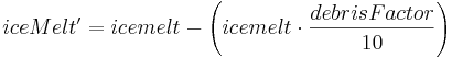
The ice melt is further adapted by the debris covered factor. Because the glaciers in the Dudh Kosi river basin are in general debris cover, a simple segregation method is applied to identify debris-covered glaciers based on slope. If the slope is higher than 30 degrees, the gravels, stones and pebbles are rolled down and the glacier is regarded as a clean glacier. The slope lower than this threshold is suitable for the accumulation of debris on top of glaciers. By using this approach, about 77 percent of the glaciers are estimated as debris-covered glaciers. According to Mool (2001a), about 70 percent of the glaciers in the Dudh Kosi river basin are valley types. One of the most common characteristics of glaciers located in the Himalayan region is the presence of debris material. In general, valley glaciers are debris-covered in the Himalayan region (Fujji 1977; Sakai2000}. It can be assumed that the debris-covered glacier areas estimated by this approach are fairly representative and adequate for purposes of this modelling application.
The presence of debris affects the ablation process. Supra-glacial debris cover, with thickness exceeding a few centimeters, leads to considerable reduction in melt rates (Oestrem 1959; and Mattson 1993). According to (Oestrem 1959) the melt rate decreased when the thickness of the debris cover was more than about 0.5 cm thick. The report further mentioned that not only the melting will be slower under the moraine cover, but also the ablation period will be shorter for the covered ice. The clean glaciers as reported on the Tibetan Plateau have higher retreat rates. (Kayastha 2000) studied the ice-melt pattern in the Khumbu glaciers (Dudh Kosi river basin where the J2000 model is being applied) and found that the debris ranging thickness from 0 to 5 cm indicates that ice ablation is enhanced by a maximum at 0.3 cm. Therefore, when a glacier is covered by debris, the ice melt is reduced. Using the calibration parameter (debrisFactor), the effects of debris cover on melt is controlled as follows.
The icemelt is further adapted with the slope and aspect of the particular glacier HRU. Routing of glacier melt is made separately for snowmelt, ice melt and rain runoff using the following formula:

where:
snowmelt = total snowmelt during the time step (mm/day)
meltRest-1 = outflow of reservoir during the last time step
kSnow = storage coefficient (recession constant) for reservoir
A similar routing procedure is applied for ice melt and rain runoff with a different recession constant (kIce) and (kRain). It is assumed that the routing of rain runoff is faster than that of ice and snow.
In reality, snow is stored in the accumulation zone of high-altitude areas. The snow is transported to low-altitude by wind, avalanches and gravity. As snow gets buried under new snow, it is gradually converted into firn and eventually into glacier ice. This ice flows by gravity downstream towards the ablation zone as glaciers (Jansson 2003). However, such dynamic processes of snow transformation and transportation are not included in the glacier module of the J2000 model. Therefore, some part of the precipitation is always stored as snow in the accumulation zone of high-altitude areas. To compensate for this long-term storage process, a constant glacier layer is used as a surrogate which provides melting from glacier ice.
Soil water module
The description of the soil water module as described in model source code is provided here which is primarily based on the technical documentation of the J2000 model (Krause, 2011).
In the soil module separate soils are represented according to their pore volumes. The pore storage which can occur in the soil are classified in the literature as follows (e.g. (Scheffer & Schachtschabel 1984)):
- The water stored in fine pores (< 0.2 μm diameter, pF > 4.2, corresponds to the permanent wilting point - PWP) is so strongly bound due to its adsorption powers that it is not at all available for runoff generation.
- The water stored in middle pores (diameter 0.2 to 50 μm, pF 1.8 to 4.2, corresponds to usable field capacity -nFk) is hold against gravity due to its adsorption powers. It can be extracted from the soil almost exclusively by using suction potential.
- The water stored in coarse and macro pores (> 50 μm diameter, pF > 1.8, corresponds to air capacity - Lk) is subject to gravitation and can be kept in the soil for only a short period of time (1 to 2 days according to (Scheffer & Schachtschabel 1984).
The water stored in the fine pores can be neglected during the modeling as it is not available for evaporation or flow processes according to the above-mentioned specification of the pore volumes due to the constant binding. Hence the modeling abstraction of the soil is carried out by two parallel and connected storage in the model J2000: one storage which corresponds to the middle pore storage volume (hereinafter referred to as MPS) and which can only be emptied by evaporation and another storage which represents the volume of the large and macro pore storage (hereinafter referred to as LPS) and which is the source for the actual runoff.
The figrue below shows the imporatant hydrological processes within the soil zone. It can be seen that an infiltration storage precedes the soil storage which contains net precipitation and water resulting from snow melt. From this storage the water is distributed to both soil storage where remaining water is cached in the depression storage in case of exceeding a maximum infiltration capacity of the corresponding soil or a saturation of the large pore storage. Emptying the depression storage is done by evaporation, the generation of surface runoff and/or seepage at a later point in time. Emptying the middle pore storage is done by evapotranspiration, emptying the large pore storage by generating interflow or by groundwater recharge. In addition, at the end of the time step a certain amount of the water stored in large pores can be transferred to the middle pore storage. The middle pore storage can, in addition to this water amount and to the infiltration, receive water from the saturated zone due to capillary rise. These individual processes are explained in detail below, however the parameterization of the soil module is discussed beforehand.

Infiltration
The first process which contains the water resulting from the snow melt and from net precipitation is infiltration. Whether water can seep away entirely or whether it is stored for a short time at the surface and whether it generates depression storage at this place or surface runoff, is subject to the infiltration capacity of the corresponding soil. The infiltration capacity is calculated by a simplified method which is suitable for daily time steps. It is based on the assumption that infiltration capacity is on the one hand subject to water saturation in the soil and on the other hand it cannot exceed a certain threshold value, a maximum infiltration rate. If this maximum infiltration rate is set to a constant mean value for the whole year, there are two problems, at least for two special cases:
- In convective precipitation with high intensities and short duration. Often the infiltration capacity of the soil is exceeded since much water comes to the soil within a short time although the precipitation amount for the whole day would not imply this.
- In snow melt runoff from the snow cover. Although water is released in a quite continuous manner, the soil behaves like a sealed area since it is partly or completely frozen or since water runs off within the snow cover without having the chance to seep away.
In order to take these special cases into account, at least rudimentarily. Two threshold values can be indicated in addition to the "standard value". Since special case 1 occurs mainly in summer months, a threshold value can be specified for summer half year. This threshold value serves to take into account thundershowers with high intensity within a short time which occur mainly during summer months. The second threshold value is applied if the modeled unit is covered in snow. Using this value the reduced infiltration capacity of the soil with a partly or completely frozen surface is considered. At the same time this value can be used to take into consideration the runoff of melt and precipitation water within the snow cover. The third value represents the standard case and therefore holds for the winter half year and for entities without snow cover.
The threshold values which are to be determined by the user (soilMaxInfSummer, soilMaxInfSnow, soilMaxInfWinter referred below in the equation as soilMaxInf1,2,3) are weighted during the modeling with the relative saturation deficit of the soil (δsat). The resulting maximum infiltration rate ( Infmax) then calculated according to:
![Inf_{max} = soilMaxInf_{1, 2, 3} \cdot (1 - satSoil) \,\,\, [mm/d]](/ilmswiki/pt/uploads/math/3/b/9/3b939f74b7706c0442beaea14323c701.png)
The relative water saturation of the soil can be calculated using:
![soilSat = \frac{actMPS + actLPS}{maxMPS + maxLPS} \,\,\, [mm/d]](/ilmswiki/pt/uploads/math/f/5/7/f579c809b43d999370938d41e3270fd5.png)
If the water amount of precipitation and snow melt for the infiltration exceeds the calculated maximum infiltration rate, the excess is transferred to the depression storage and cached there. The resulting, actually seeping water amount (Infact ) is distributed among the soil storages. The amount of water which is in every soil storage is subject to the saturation deficit of the middle pore storage (MPS) and is calculated using the calibration parameter soilDistMPSLPS as follows:
The large pore storage (LPS) receives remaining water according to:
![MPS_{in} = Inf_{act} \cdot \frac{1 \cdot soilDistMPSLPS}{satMPS} \,\,\, [mm]](/ilmswiki/pt/uploads/math/d/4/f/d4f19c38bcd2ce7f14160a02f7c80f21.png)
The large pore storage (LPS) receives remaining water according to:
![LPS_{in} = Inf_{act}-MPS_{in} \,\,\, [mm]](/ilmswiki/pt/uploads/math/8/9/d/89d0c15e5e2c36394e6ae80e87ba965c.png)
Due to the water distribution according to these equations the middle pore storage works like a sponge and its potential of taking water increases with increasing dehydration. However, a certain amount always remains in the large pore storage. The weighted distribution has the advantage that even in dry soils, especially during the summer months, part of the infiltrated water can run off fast. If the water was not
distributed, interflow could only occur after saturating the middle pore storage, i.e. after achieving usable field capacity. Various investigations showed that large and macro pores can also achieve runoff if there is no water saturation in the soil.
Other special cases of infiltration occur with sealed areas and water areas. For water areas the water which is actually available for infiltration is transferred to an individual storage which can only be emptied by evaporation. In sealed areas only a certain amount of water on the surface seeps away subject to the degree of sealing (e.g. 25% with degree of sealing > 80% and 60% with degree of sealing < 80% according to (Wessolek 1993). The remaining part contributes to the total runoff in the form of surface runoff. This is considered by using corresponding coefficients (soilImpGT80, soilImpLT80) which have to adjusted by the user.
The depression storage
As represented in the description of infiltration above, the water amount which exceeds the maximum infiltration rate of the soil is transferred to the depression storage. This also applies if the soil is completely water-saturated and no infiltration can take place. The water which is stored in the depression storage runs off partly as surface runoff. The maximum amount in mm m{-2} which can be kept as depression storage on the individual are has to be indicated during model parameterization. According to Maniak (1997) the maximum depression storage lies between 0.6 and 8.0 mm per m² subject to the specific land use. Since this variable has a relatively low impact on the dynamics of runoff lines (Maniak 1997), the maximum depression storage is set to a lump value and is not differentiated according to the land use. As the depression storage is only important in rather lowly-elevated locations, the maximum depression storage is weighted using the slope of the specific area. As, according to Maniak (1997), the maximum depression storage decreases by 50% from 4-6 % slope, the volume of the depression storage halved for areas exceeding this slope. If the maximum depression storage is exceed on an area, spare water is released as surface runoff.
The middle pore storage
The water stored in the middle pores of the soil is held against gravity due to the adsorption powers. This means an active soil water potential is required in order to extract water from the middle pore storage. The potential for such a soil water suction is made available by evaporation. Two different cases have to be distinguished: the direct evaporation from the soil surface and the evaporation caused by transpiration of the vegetation cover. The direct evaporation of the soil surface is comparably low since only a few millimeters of dry soil can cause an effective isolation of the underlying layers regarding the evaporation. This isolation is shorted out by the roots of the vegetation cover, which makes a consistent exhaustion of water stored in the middle pores possible by transpiration. With increasing dehydration of the soil the actual evaporation decreases significantly in relation to potential evaporation. For simulating this reduction an established linear approach ([Gurtz et al. 1997]; [Schulla 1997]; [Uhlenbrook 1999]) is used or a nonlinear approach which has been developed for the model is applied.
When using the linear approach it is assumed that the real evaporation equals potential evaporation until a specific water saturation is achieved. When the value goes below this water saturation, the real evaporation decreases consistently in relation to potential evaporation until it is zero when reaching the permanent welting point (= complete emptying of nFk). As threshold value (soilLinRed) for this specific water saturation values between 0.8 to 0.6 are mentioned in the literature ([Gurtz et al. 1997]; [Menzel 1997]). This threshold value and the actual water saturation of the middle pore storage M (satMPS) is used to calculate a reduction factor (RF):

The large pore storage
The water which is in the large pore storage (GPS) is subject to gravitation and is therefore considered as the source of actual flow processes and runoff generation of the soil in J2000. Filling the storage is done by the infiltration amount which remains after subtracting the inflow to the middle pore storage.
The different runoff behavior of different soils is reflected very well by the pore volumes which have been defined beforehand. Clayey soil has a relatively high proportion of fine and middle pores, whereas sandy soil has a comparably high amount of large pores. The generation of lateral and vertical runoff and the amount of precipitation is correspondingly different. The water which is stored in rather clayey soil contributes less to lateral and vertical runoff, under the same conditions (e.g. vegetation cover, slope etc.), than does rather sandy soil. In contrast, the water amount available for evaporation is significantly higher in clayey soils than in sandy soils. Clayey or silty soil, which lies between the above-mentioned soils according to their pore size, has the best water storage capacities since it has the highest amount of middle pores.
The water amount which generates runoff from the large pore storage in the time step is subject to the relative water saturation of the entire soil (LPSsoil) and is calculated according to:
![Q_{LPS} = (Sat_{soil})^\alpha\ \cdot LPS_{act} \,\,\, [mm]](/ilmswiki/pt/uploads/math/c/2/b/c2be8c34040c3bcbdec6412a4b8c089d.png)
with:
QLPS: Outflow from LPS [mm]
Satsoil: Relative water saturation of the soil at location [-]
α : calibration coefficient [-]
The advantage of this non-linear outfall function is that much less water runs off in low areal humidity than if it were a linear drain function. The common behavior of catchment areas which generate much more and faster runoff when there is high soil moisture (Baumgartner & Liebscher 1990; Dyck & Peschke 1995) than when there is low soil moisture (assuming the same precipitation amount) can be better displayed using an outfall function.
The gravitation water flowing out from the LPS (QLPS ) is distributed among three different target storage. A certain amount goes to the middle pores and is stored there for a longer period of time, a second part percolates into the groundwater storage (vertical component) and the remaining amount provides the source for interflow (lateral component). The size of the components is subject to soil-physical parameters (especially kf values) and the slope of the corresponding HRU. Therefore, it is assumed in the model that the slope area generates much interflow, whereas in almost evenly situated locations the percolation into the groundwater is the main component. The amount which goes from large pores into middle pores is, however, subject to the saturation of the middle pore storage. In order to determine of runoff amounts the slope and two kf values have to be specified for each HRU: The kf value of the soil horizon with the lowest permeability and the kf value of the overlying horizon.
Percolation and interflow generation
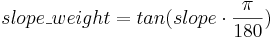
A certain amount of available gravitation water seeps through the entire soil and contributes to groundwater recharge. In the model presentation of the J2000 this percolated amount is represented as dependent on the slope of the corresponding HRU. The slope influences the percolation in that inclined areas have a higher amount of gravitation water as lateral runoff from unsaturated zones, i.e. the groundwater recharge is less in these areas than in evenly situated locations. The influence of the slope is taken into account with a gradient according to the following equation:
![grad_{perc} = (1 - tan \alpha)^\beta\ \,\,\, [-]](/ilmswiki/pt/uploads/math/b/4/7/b4751c719100071c7cfcb8c8dc86c1c6.png)
α: slope of the corresponding HRU [degree]
β : shape parameter, calibration coefficient [-]
Using this equation the relation between vertical and lateral runoff is determined which can be adapted to the conditions in the catchment area with help of the calibration coefficient β. In addition, with this calibration coefficient the slope resulting from coarse-grained models which is systematically too low can be enhanced.
The water amount which is available for percolation is calculated according to:
![Perc_{pot}= grad_{perc} \cdot Q_{LPS} \,\,\, [mm]](/ilmswiki/pt/uploads/math/2/6/2/262403489d60dde0cbfcb4044d9fd1a8.png)
This percolation rate is then set against the calibration coefficient soilMaxPerc which describes the maximum percolation rate per time step.
And for the interflow Interflow(RD2):
![Interflow = 1- grad_{perc} \cdot Q_{LPS} \,\,\, [mm]](/ilmswiki/pt/uploads/math/1/3/4/1349901955816bcc2573cb7f8d4f5855.png)
Runoff detention
Both runoff components, direct runoff (RD1) and interflow (RD2) are delayed in time in order to take into account the areal expansion of the spatial model entity. The detention takes place using corresponding retention coefficients (soilConcRD1, soilConcRD2). The detention is calculated according to:
![RD1 = \frac{1}{soilConcRD1} \cdot RD1{gen} \,\,\, [mm]](/ilmswiki/pt/uploads/math/6/6/6/6662a9767b6f79ee415d0e5c73ca5ffb.png)
![RD2 = \frac{1}{soilConcRD2} \cdot RD2{gen} \,\,\, [mm]](/ilmswiki/pt/uploads/math/6/a/a/6aaa9cf5de9b80ce05d719a3f0c6e790.png)
Nepal (2012) suggested that in the case of RD1, the delayed time may be different during high-flow periods due to non-linear behavior of a catchment. Beven (2001a) highlighted that the non-linear responses primarily exist due to two causes. The first reason is the antecedent condition when the relationship between rainfall and runoff is generally considered to be nonlinear because the wetter the catchment prior to a unit input of rainfall, the greater the runoff that will be generated. Second, a non-linearity exists also due to change of velocity with discharge. Average flow velocities increase with the flow with both surface and subsurface flow processes. Faster flow velocities mean that the runoff will reach a measurement point in the stream-channel flow system more quickly. In case of high precipitation events (such as during the monsoon season in the study area) which are responsible for high flood peaks, a high degree of non-linearity is noted. During those events, the soil becomes saturated by the initial rainfall events and a higher rainfall-runoff coefficient is likely after some periods of rainfall. These typical conditions have been taken into account by introducing a new parameter into the J2000 modelling system. The new parameter (concRD1Flood) is used by the model when the RD1gen crosses a threshold value (RD1FloodThreshold) provided by a user. The value of (concRD1Flood) should be lower than concRD1 because it produces higher RD1 output flow.
![RD1_{flood} = \frac{1}{soilConcRD1Flood} \cdot RD1{gen} \,\,\, [mm]](/ilmswiki/pt/uploads/math/7/5/6/756d5cee753961b4049cc4432e6232fe.png)
Diffusion
At the end of the time step a deficit of the middle pore storage (MPS) resulting from evaporation be balanced out by water from the large pore storage (LPS). This diffusion ( diff) is carried out using the calibration coefficient soilDiffMPSLPS according to:
![diff = actLPS \cdot (1-e\frac{-1\cdot diff }{satMPS}) \,\,\, [mm]](/ilmswiki/pt/uploads/math/7/2/6/726e9e78278eb2ae7cda9c3829e5f137.png)
For more information see also: [Baumgartner & Liebscher 1990], [Dyck & Peschke 1995], [Gurtz et al.
1997], [Maniak 1997], [Menzel 1997], [Scheffer & Schachtschabel 1984], [Schulla 1997], [Uhlenbrook
1999], [Wessolek 1993]
Groundwater module
The model structure of the groundwater module in J2000 allows the presentation of the groundwater runoff of all geological formations existing in the catchment area by considering their storage and runoff behavior. Those formations have to be parameterized separately. The geological units are subdivided into the upper groundwater storage (RG1) in the weathered loose material with high permeability and short retention time and the lower groundwater storage (RG2) in the matrix and in fissures and ravines of the bedrock with low permeability and long retention time. Correspondingly, two basic runoff components are generated, a fast one from the upper groundwater storage and a slow one from the lower groundwater storage. Filling the groundwater storage results from the vertical runoff component of the soil module (percolation), emptying can be done by the lateral underground runoff components and the capillary rise on the unsaturated zone. The parameterization of the groundwater storage is carried out using the maximum storage capacity of the upper (maxRG1) and the lower groundwater storage (maxRG2) as well as the retention coefficient for both storages, (kRG1) and (kRG2). The maximum storage capacity can be estimated by multiplying the part of the underground chamber with the thickness of the individual storages per m² standard area. Both parameters have to be defined for every geological unit separately and have to be saved in the corresponding parameter file. The following table shows an example of such a parameter file.
The first process to be calculated is the capillary rise. It is assumed that this action takes place in the slow groundwater storage RG2. The calculation is done using the actual storage amount actRG2, the humidity deficit (deltaSoilStor) or the relative saturation (satSoilStor) in the upper soil and the calibration parameter gwCapRise. Capillary rise is calculated if the current storage amount of the groundwater storage is higher than the soil humidity deficit and the calibration parameter gwCapRise is above zero. By putting it to zero the capillary rise can be prevented.
If capillary rise is calculated, first the rise rate inSoilStor is calculated:

It is then extracted from the groundwater storage RG2 and added to the upper soil water storage. After calculating the capillary rise the lateral inflow is considered. Hence, both inflow components inRG1 and inRG2 are added to the corresponding storages actRG1 and actRG2. If the maximum storage capacity is exceeded, surplus water is directly given to the runoff component.
The allocation of the percolation from the upper soil is carried out according to the slope of the specific model entity and a calibration coefficient (gwRG1RG2dist) in the following steps. First, the influence of the slope is considered:

Then the percolation rate is allocated:


The potential inflows are calibrated against the corresponding current storage. If RG2 cannot take the inflow pot_RG2 completely, the surplus is transferred to pot_RG1. If RG1 cannot take pot_RG1, the surplus is given to gwExcess. According to the model’s concept this variable can be assigned to a specific runoff component.
The calculation of water discharge is carried out according to the current storage amount in form of a linear storage-outflow function. The storage retention coefficients (kRG1, kRG2), which are considered as the time water rests in the specific storage, are a factor of the current storage volume (actRG1 and actRG2) used for the calculation of the groundwater outflow (outRG1 and outRG2) as follows:
![outRG1 = \frac{1}{gwRG1Fact \cdot kRG1} \cdot actRG1 \,\,\,[mm]](/ilmswiki/pt/uploads/math/3/7/5/375a83a0310197488cf0e4e37bd210f6.png)
![outRG2 = \frac{1}{gwRG2Fact \cdot kRG2} \cdot actRG2 \,\,\,[mm]](/ilmswiki/pt/uploads/math/3/2/9/32984394f92f6fc1be6c8418ca6ca51a.png)
The groundwater dynamics can be calibrated using parameters gwRG1Fact and gwRG2Fact.
Routing module
The J2000 module has two different routing components. The lateral routing component serves to simulate lateral flow processes in the catchment area until the water finally reaches a preflooder segment or a reservoir. In order to do so, the individual runoff components which are generated in the model entities are transferred to the corresponding recipient. This component does not have any calibration parameters.
The reach routing component is used for modeling flow processes in the on-site preflooder network of the catchment area. First, separate reaches have to be parameterized. The individual parameters which have to be assigned, are length in meters, slope in %, the mean width in meters and the reach roughness according to Manning-Strickler. Those are stored in a parameter file which is read by the model and by which the corresponding objects are generated. Additionally, the file contains information on the structure of the flow topology by noting the ID for every reach into which it empties. The reach representing the catchment outlet has to contain the ID 0.
The individual reaches receive water by neighboring spatial model entities and upstream reaches. In the reach, a velocity for water amount is calculated and then a certain amount is given to the next downstream reach based on the velocity and the length of the on-site preflooder. For the calculation a rectangular cross section is assumed to simplify matters. Although the complete amount of water is routed, the relative amounts of the individual runoff components are maintained, so they can be considered separately anytime and in every reach.
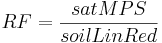
The module describes flow processes in the channel by using the kinematic wave approach and the calculation of velocity according to MANNING & STRICKLER. The only parameter that has to be set by the user (TA)(also referred as flowRouteTA) is a routing coefficient. It represents the runtime of the runoff wave which moves in the channel until it reaches the catchment outlet after a precipitation event. Its value is required for the calculation of the restraint coefficient (Rk) together with velocity of the river (v) and flow length (fl):
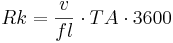
Before doing so, the velocity (vnew) has to be determined using the roughness factor by Manning (M), slope of the river bed (l) and the hydraulic radius (Rh). The hydraulic radius is calculated using the drained cross section (A) of the reach which results from the flow rate (q), velocity (v) and river bed width (b). For this approach, a start velocity (vinit) is assumed which is then iteratively adjusted with regard to the new calculated velocity (vnew) until both velocities differ in a value smaller than 0,001 m s^{-1}:
![Rh = \frac{A}{b + 2 \frac{A}{B}} \,\,\,\,[m]](/ilmswiki/pt/uploads/math/3/c/c/3cc797fe2d82ddcee5436562ff40c79c.png)
with:
![A = \frac{q}{v_{init}} \,\,\,\,[m^2]](/ilmswiki/pt/uploads/math/3/3/d/33d139a9fef2aeca40b23983714aba3c.png)
![v_{new} = M \cdot Rh^{\frac{2}{3}} \cdot l^{\frac{1}{3}} \,\,\,\,[m^3/sec]](/ilmswiki/pt/uploads/math/6/a/7/6a75983b418068db72ed6109cfca1993.png)
![q = q_{act} \cdot e^{\frac{-1}{Rk}} \,\,\,\,[m^3/sec]](/ilmswiki/pt/uploads/math/d/c/5/dc58c7086482d6c68daf4fe60b3cefec.png)
Finally, the amount of water of the corresponding reach ( ) is calculated which goes to the runoff ( ) using the runoff restraint coefficient ( ) which has been generated.
The higher the assumed value of TA, the faster does the runoff wave move within a certain time span and the less water remains in the channel.