OBIS: Time series data
The section time series data is one of the core features of OBIS. OBIS allows the management, visualization and download of time series data. The section "Time series data" gives first an overview of all datasets. The measured data are directly linked to the stations, where they have been measured.
Contents |
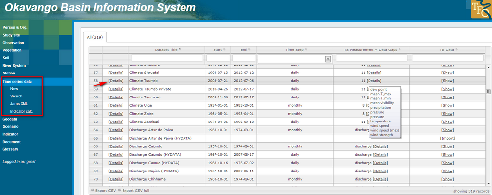
View list of available datasets
On the screen most important information are listed:
- Dataset title consists of measured parameter and station name, e.g. "Climate Benguela"
- Start of time series (yy-mm-dd)
- End of time series (yy-mm-dd)
- Time step, e.g. daily, monthly
- TS Measurement + Data Gaps, e.g. precipitation, discharge
- TS Data contains the link to access the data [show]
Metadata
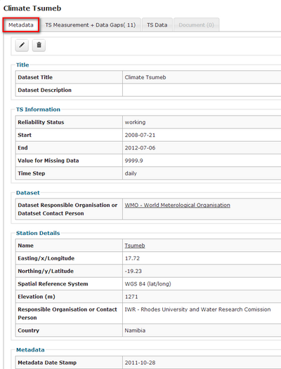
With a click on "Details" you can see all data linked to the dataset. First metadata are listed. They are grouped in Title, Time series information, Dataset and Station details.
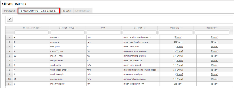
If you chose the register "TS Measurements + Data Gaps" timeseries are listed. In the example Luanda eight time series are available.
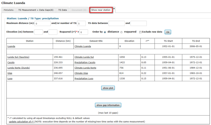
Show near stations
RBIS allows to search for nearby stations to include time series from neighbouring stations in various calculations. Often time series have data gaps or need to be extended, i.e. extrapolated. In both cases -interpolation and extrapolation- nearby stations or rather their time series data are used. The table lists nearby stations, their distance, dataset title, elevation, coefficient of determination (rsquared) and start and end date of time series. You can order the results by distance or rsquared. OBIS allows further to search for specific stations, e.g. nearest stations, high coefficients of determination or a specific time frame. For each time series it is possible to conduct a gap analysis. A plot can be generated, where gaps greater than 5 days are marked in red.
View and download time series data
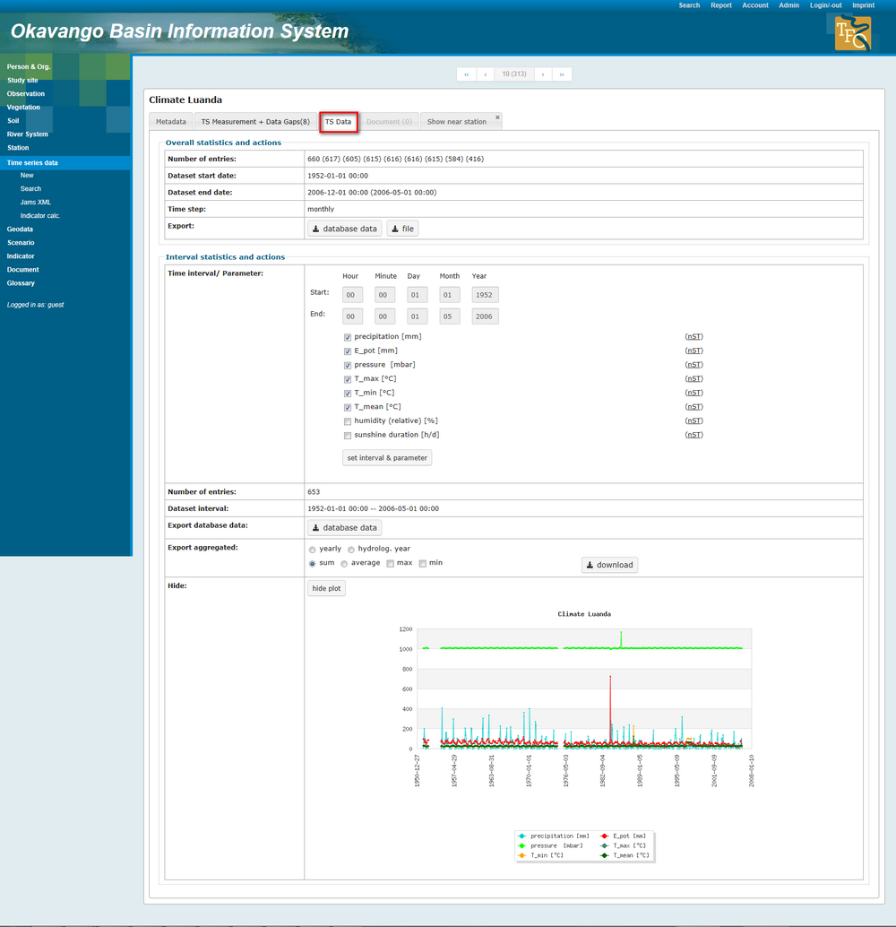
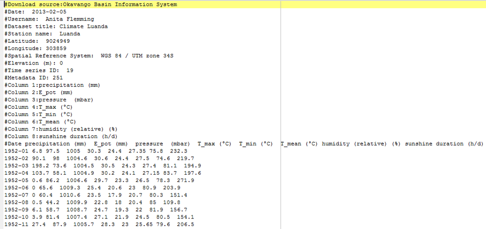
The section "overall statistics and actions" lists the number of entries in total and in brackets the number of entries for each parameter. You get an overview of the completeness of the time series or number of gaps. Start and end date of the time series is shown. For the export of data you have two possibilities: If you are interested in the entire dataset, use the download link "database data" and you get a txt-file containing all data and metadata. The example "climate Luanda" file opened in an editor (see figure below), shows you station information and time series information, lists the parameters in their correct order and gives you the monthly data. Using this download link you get the data as they are stored in the database (no default values, no date gaps). Using the download link "file" the original file will be exported as it has been uploaded to the database.
In the section "Interval statistics and actions" you have the possibility to view the time series data in a plot. You can set a time interval and parameters of interest. Therefore enter the time interval in the entry fields, activate the checkboxes of the parameters of interest and confirm the selection by clicking "set interval & parameter". By clicking on the link "show plot" a graph appears visualizing time series data for the timeframe and parameters selected before. By clicking on the link "database data" you get the time series for this respective timeframe and parameters. You can also chose the function "Export aggregated" for download. This feature allows to export e.g. yearly data, average data, max or min values or sum. Tick the checkboxes of the required output and click on "download".
Visualization of a txt-file in PSPad (download via the link "database data")
Interpolation of gaps
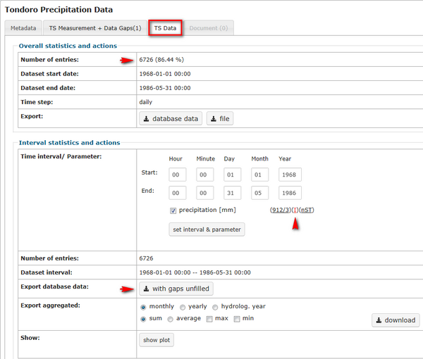
Some time series show data gaps. They were indicated in the first row in the table. The percentage next to the number of entries shows the completeness of the time series.
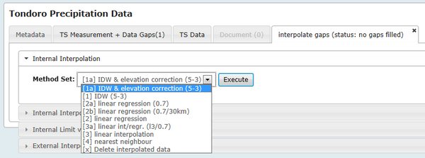
RBIS includes different interpolation methods. The methods are explained in the section "Internal Interpolation Method Set". You can chose between following internal interpolation methods:
- inverse distance weighting (& elevation correction)
Inverse distance weighted methods are based on the assumption that the interpolating surface should be influenced most by the nearby points and less by the more distant points. The interpolating surface is a weighted average of the scatter points and the weight assigned to each scatter point diminishes as the distance from the interpolation point to the scatter point increases.
[1] IDW (5-3) Inverse distance weighting (IDW) (max 5 stations - min 3 stations are used) [1a] IDW & elevation correction (5-3) Inverse distance weighting (IDW) with elevation correction (max 5 stations - min 3 stations are used). If elevation is incorrect (not given) only IDW is used.
- linear regression
Linear regression is an approach to modeling the relationship between a scalar dependent variable y and one or more explanatory variables denoted X. The case of one explanatory variable is called simple regression. More than one explanatory variable is multiple regression.
[2] linear regression with the values of the station with the best r² is used. [2a] linear regression (0.7) Linear regression with the values of the station with the best r² in a radius of 10 stations is used if r² is at least 0.7 or greater.
- [2b] linear regression (0.7/30km) Linear regression with the values of the station with the best r² in a radius of 10 stations which is at least 0.7 or greater is used. The maximum distance of this station is 30km.
- linear interpolation
Linear interpolation is a method of curve fitting using linear polynomials.
[3] linear interpolation [3a] linear int/regr. (l3/0.7) Linear interpolation is used if gap length is not more than 3. Gaps greater 3 are closed by linear regression with the values of the station with the best r² in a radius of 10 stations is used if r² is at least 0.7 or greater.
- nearest neighbor
Nearest-neighbor interpolation (also known as proximal interpolation or, in some contexts, point sampling) is a simple method of multivariate interpolation in one or more dimensions. Interpolation is the problem of approximating the value of a function for a non-given point in some space when given the value of that function in points around (neighboring) that point. The nearest neighbor algorithm selects the value of the nearest point and does not consider the values of neighboring points at all, yielding a piecewise-constant interpolant.
[4] nearest neighbour
The user selects one method or can chose a combination of interpolation methods. In addition the user has the possibility to define rules for the application of the method by clicking on "Internal Interpolation Method Set". A description of the method is given here.
