Model oupt
(Created page with " In addition, the model also provides the different efficiency results at the end of the model run. For this, the 'TSVisualization' component of the JAMS builder has to be expa...") |
|||
| Line 1: | Line 1: | ||
| − | + | In addition, the model also provides the different efficiency results at the end of the model run. | |
| − | + | ||
For this, the 'TSVisualization' component of the JAMS builder has to be expanded (click + and - sign on the left side to expand and reduce) as shown in Figure below. The existing TS plots will be shown. The new plot can be created by using the existing plot. Drag one of the existing plots (example, Glacier contribution) and hold CTRL key (a + sign will appear) and leave both the keys. The new plot will appear with the new name (Glacier contribution_1). From the right window, the name and the values of the new plot can be changed. Mainly, four things has to be changed in the new plot. | For this, the 'TSVisualization' component of the JAMS builder has to be expanded (click + and - sign on the left side to expand and reduce) as shown in Figure below. The existing TS plots will be shown. The new plot can be created by using the existing plot. Drag one of the existing plots (example, Glacier contribution) and hold CTRL key (a + sign will appear) and leave both the keys. The new plot will appear with the new name (Glacier contribution_1). From the right window, the name and the values of the new plot can be changed. Mainly, four things has to be changed in the new plot. | ||
Latest revision as of 09:01, 1 October 2012
In addition, the model also provides the different efficiency results at the end of the model run.
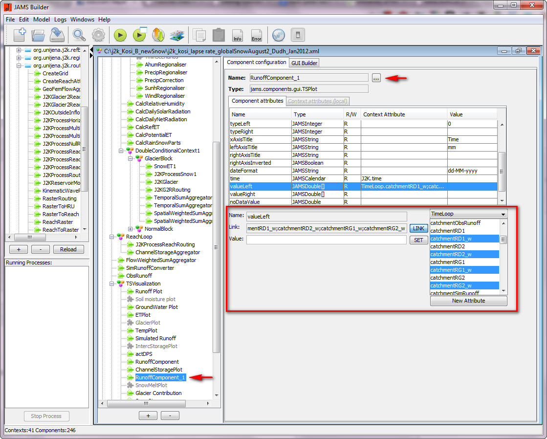
For this, the 'TSVisualization' component of the JAMS builder has to be expanded (click + and - sign on the left side to expand and reduce) as shown in Figure below. The existing TS plots will be shown. The new plot can be created by using the existing plot. Drag one of the existing plots (example, Glacier contribution) and hold CTRL key (a + sign will appear) and leave both the keys. The new plot will appear with the new name (Glacier contribution_1). From the right window, the name and the values of the new plot can be changed. Mainly, four things has to be changed in the new plot.
1. Change the name of the component. Click the [...] box on the right hand side of the 'Name'. This will bring a new window and you can change the name of the new plot.
2. Provide new names for the legend used in the plot. Click on the 'titleLeft' row and change the name of the legends under 'Value' window. In case of more than one legend, seperate the name by semicolon.
3. Provide colors to the legends. Click 'colorLeft' row and change the color name under 'Value' window.
4. Provide value for the legends. When 'valueLeft' row is clicked, the window below is activated. The value can be choosen from Timeloop. Use CTRL key to choose more than one value.
Alternatively, this information can be changed by editing the model xml file which has been explained below.
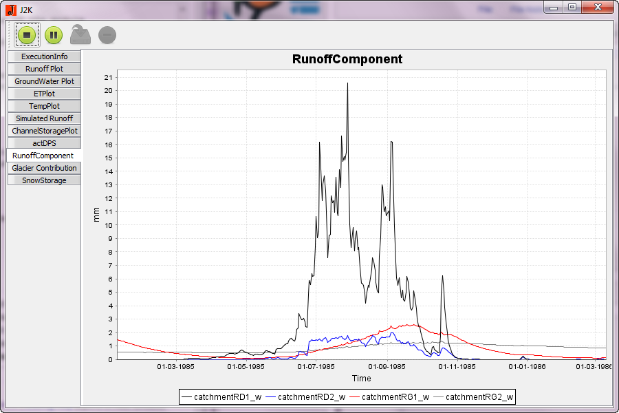
With these lines in xml file as shown in figure below, users can define which output files they wish to see as a plot/graph. In the figure below, four different runoff components are displayed.
After defining the plot, users also need to define a line in a 'Plot & Maps' component to bring it in the JAMS framework. For example: The first line is dedicated to display the Runoff plot.
The Runoff Plot will appear in Plots & Maps group in JAMS launcher after loading the xml file in JAMS, which users can tick on/off to display as a graph.
After running the model, users can see the graph of different runoff components as provided below:


