OBIS: Edit Time series data
(→Data gaps) |
(→Find nearby stations) |
||
| Line 73: | Line 73: | ||
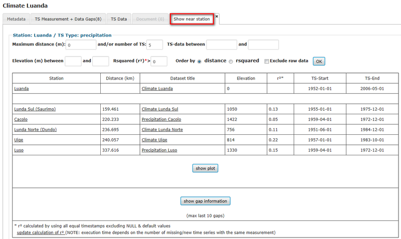
The table lists nearby stations, their distance, dataset title, elevation, coefficient of determination (rsquared) and start and end date of time series. If the number of your listed datasets is less than 8, a plot can be generated, where all data gaps are marked in red. This is very helpful to identify possible neighboring stations to fill data gaps. | The table lists nearby stations, their distance, dataset title, elevation, coefficient of determination (rsquared) and start and end date of time series. If the number of your listed datasets is less than 8, a plot can be generated, where all data gaps are marked in red. This is very helpful to identify possible neighboring stations to fill data gaps. | ||
| − | '''Show gap information''' will generate a list as it would be generated during the interpolation process (see [[OBIS:_Time_series_data#Gap_filling_toolbox|Gap filling Toolbox]]). In comparison to the above list in addition the time interval and unit have to be equal and data values have to be available in respect to each single gap interval.[[File:OBIS_Timeseries_ShowNearStation.png|800px|]] | + | '''Show gap information''' will generate a list as it would be generated during the interpolation process (see [[OBIS:_Time_series_data#Gap_filling_toolbox|Gap filling Toolbox]]). In comparison to the above list in addition the time interval and unit have to be equal and data values have to be available in respect to each single gap interval. |
| + | |||
| + | [[File:OBIS_Timeseries_ShowNearStation.png|800px|]] | ||
== Gap filling toolbox == | == Gap filling toolbox == | ||
Revision as of 14:32, 13 March 2013
Time series data stored in the database can be edited or deleted by clicking on the icons ![]() to edit or
to edit or ![]() to delete data. You have to click in the time series data overview on the link "Details" of the respective dataset you wish to edit.
to delete data. You have to click in the time series data overview on the link "Details" of the respective dataset you wish to edit.
- In the metadata section of the dataset you have the possibility to edit the data in case you have the required authorization rights. For editions the data entry form appears. Now you can edit the entry fields. If you want to clear all entries use the button "Reset". Finally click on "Submit" to update the data entry form. You are getting informed when processing has been successful.
- A datasheet can only be deleted completely when no other data are linked to it. You may only delete a data sheet having no dependencies on other data. After clicking the delete button you are getting informed when deletion has been successfully.
Contents |
Add new data
If you wish to add new data to a time series, select first the dataset. Click on "Details" in the row of the dataset where you want to add data. Go further to the section "TS Data". At the end of the form you will find the button "add data".
Form "Upload timeseries data"
The form "Upload timeseries data" appears. In this form you have to upload the input file. Then you need to select the number of columns (do not count the date column) and specify the file format, date format, values for missing data and time step. You can tick the checkbox "Time shift" if you want to use this function. It corrects the given input time. The time shift in a time interval will be corrected. The reference for shifting is the first time given. Example: 5-minutes values: 12:30 12:35 12:41 12:48 will be shifted to 12:30 12:35 12:40 12:50. Further you need to specify the used character for the beginning of a comment line.
Input file for upload
Time series should be available in a text or CSV file and should only contain data, i.e. date of measurement and values. Additional metainformation in the header needs to be set up as comment. At the end of the file (below data entries) there must not be any comment. Text files need to agree with the following rules:
- comments need to be introduced with # or *
- data needs to be listed in ascending order
- TAB serves as column delimiter (text file)
- the first entry needs to be a measurement value
- measurements needs to be numeric
- decimal delimiter is "," or "."
- data for missing entries needs to be consistent
To finish the import click "Send file". After the successful import the form for the edition of metadata will open automatically. At this stage you have to specify the type of uploaded data, e.g. Title, TS information, Dataset, Station Details... Use the link "Edit all" on top of the table if you have uploaded data with several columns to reduce efforts. The link "Edit" specifies only one column, so that you need to edit imports containing more than one columns several times.
Import of time series data
If you want to create new time series data use the subitem "New" in the section "Time series data". A blank metadata form will appear and you have to fill out the entry fields. The form consists of several section namely Title, TS information, Dataset, Station Details, Metadata and Dataset Permission. For each entry field a help is available clicking on the question mark symbol. For various entry fields you have to do a selection by using a pull down menu.
- Title: You need to give a title and a brief description of the dataset
- TS information: You have to enter the kind of data, e.g. measured or simulated, give information about the reliability, set start and end date of the time series, give a value for missing data, e.g. -9999 and set the time step (daily, monthly..)
- Dataset: Enter a responsible organisation/ person and distributor of the data. In case you want to set limitations for the use, you can do it here
- Station details: Select a station in the pull down menu. As far es known data like coordinates and elevation will be added automatically.
- Metadata: give a date stamp
- Dataset permission: select desired permission in the pull down menu (e.g. download, data on request, invisible), name an owner
Note: Please fill out as much entry fields as possible. Data are more reliable and usable when comprehensive metadata information is available.
You have the possibility to save the filled form as template by using the respective button. To save the settings done, click the button "Submit".
In a next step you can connect time series data to the metadata sheet. Pleaser refer to the Form "Upload timeseries data.
Deletion of time series data
If you wish to add new data to a time series, select first the dataset. Click on "Details" in the row of the dataset where you want to add data. Go further to the section "TS Data". At the end of the form you will find the button "Delete all data". After clicking the button you need to confirm the deletion.
Time series data analysis
Data gaps
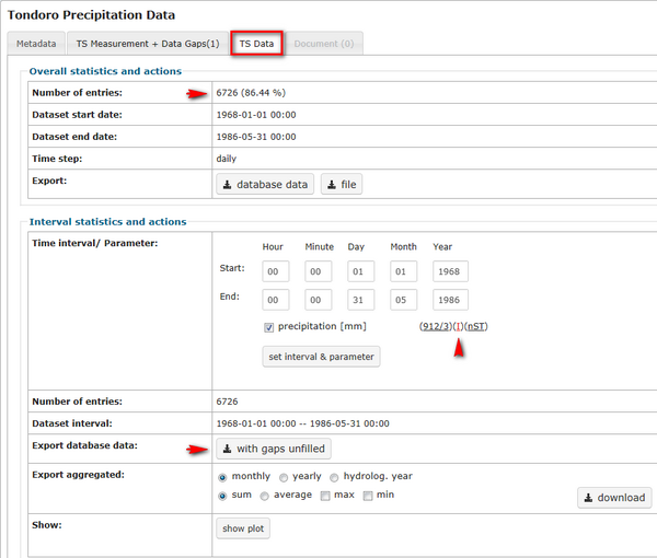
Data gaps in time series will be automatically identified during the import process. The percentage next to the number of entries in the first row shows the completeness of the time series for each parameter. In the Interval statistics section you will find below-mentioned to each parameter the number of missing values and the sum of gaps. These values are linked to the full list of data gaps. The color of the following "I" shows if data gaps are already filled (green), partly filled (blue) or not filled (red). To fill data gaps please follow the link "I". The Gap filling Toolbox will open in a new tab and provides several methods to fill data gaps.
Find nearby stations
RBIS allows to search for nearby stations with respect to one previously slected parameter (e.g. precipitation). You can search for neighboring stations by a variety of different attributes: distance (in m), elevation (in m), coefficient of determination (rsquared) and the time interval. The number of results can be limited and ordered either by distance or the coefficient of determination. To simulate the same behavior as during an interpolation process (see Gap filling Toolbox) tick on "Exclude raw data". This will exclude all time series data marked as "raw data".
Notice: Before you can use the coefficient of determination you have to calculate it. Click the link on the bottom named "update calculation of r²".
The table lists nearby stations, their distance, dataset title, elevation, coefficient of determination (rsquared) and start and end date of time series. If the number of your listed datasets is less than 8, a plot can be generated, where all data gaps are marked in red. This is very helpful to identify possible neighboring stations to fill data gaps.
Show gap information will generate a list as it would be generated during the interpolation process (see Gap filling Toolbox). In comparison to the above list in addition the time interval and unit have to be equal and data values have to be available in respect to each single gap interval.
Gap filling toolbox
Identified data gaps can be filled either by the internal rule based gap filling toolbox or externally.
Internal interpolation methods
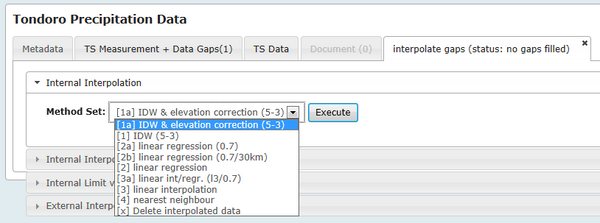
RBIS includes different internal interpolation methods. The methods are explained in the section "Internal Interpolation Method Set". You can chose between following internal interpolation methods:
- inverse distance weighting
Inverse distance weighted methods are based on the assumption that the interpolating surface should be influenced most by the nearby points and less by the more distant points. The interpolating surface is a weighted average of the scatter points and the weight assigned to each scatter point diminishes as the distance from the interpolation point to the scatter point increases.
Inverse distance weighting (IDW) uses the maximum given number of stations. If this number is not available the number is reduced to the given minimum number of stations.
[1] IDW (5-3) Inverse distance weighting (IDW) (max 5 stations - min 3 stations are used)
[1a] IDW & elevation correction (5-3) Inverse distance weighting (IDW) with elevation correction (max 5 stations - min 3 stations are used). Elevation correction is done by adjusting the values of the used stations to the elevation of the source station. These corrected values are used for IDW. If IDW with elevation correction is not possible only IDW is used instead. The default exponent is 2 otherwise it can be changed by the value of the parameter field.
- linear regression
Linear regression is an approach to modeling the relationship between a scalar dependent variable y and one or more explanatory variables denoted X. The case of one explanatory variable is called simple regression. More than one explanatory variable is multiple regression.
[2] linear regression with the values of the station with the best r² is used.
[2a] linear regression (0.7) Linear regression with the values of the station with the best r² in a radius of 10 stations is used if r² is at least 0.7 or greater.
[2b] linear regression (0.7/30km) Linear regression with the values of the station with the best r² in a radius of 10 stations which is at least 0.7 or greater is used. The maximum distance of this station is 30km.
- linear interpolation
Linear interpolation is a method of curve fitting. If two known points are given (value before and after gap), the linear interpolant is the straight line between these points. The default exponent is 2, otherwise it can be changed by the value of the parameter field.
[3] linear interpolation
[3a] linear int/regr. (l3/0.7) Linear interpolation is used if gap length is not more than 3. Gaps greater 3 are closed by linear regression with the values of the station with the best r² in a radius of 10 stations is used if r² is at least 0.7 or greater.
- nearest neighbor
Nearest-neighbor interpolation (also known as proximal interpolation or, in some contexts, point sampling) is a simple method of multivariate interpolation in one or more dimensions. Interpolation is the problem of approximating the value of a function for a non-given point in some space when given the value of that function in points around (neighboring) that point. The nearest neighbor algorithm selects the value of the nearest point and does not consider the values of neighboring points at all, yielding a piecewise-constant interpolant.
[4] nearest neighbour
screen method selection
Define rules for interpolation methods
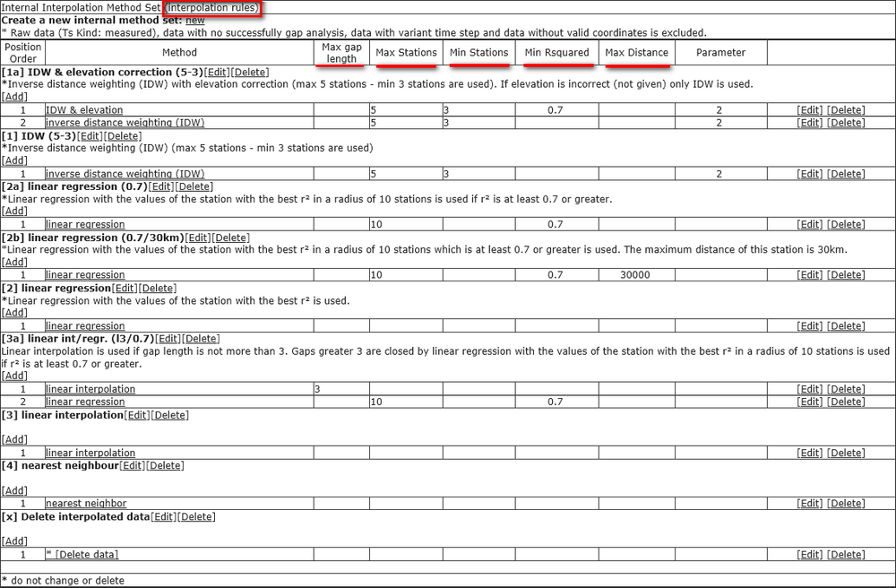
The user selects one method or can chose a combination of interpolation methods. In addition the user has the possibility to define rules for the application of the method by clicking on "Internal Interpolation Method Set". A description of the method is given here. With support of selected rules the interpolation method can be adapted. Here values can be set for the parameters: length of data gap until the method shall be applied, maximum and minimum station number, coefficient of determination r2 and maximum distance. To set a maximum length of data gap is especially recommended for the linear interpolation method as this method is not suitable for larger data gaps. If you want to change the default setting, click on the button "Edit". Default values have been set, e.g. maximum number of stations is 5, minimum nuber is 3 and the minimum coefficient for determination was set to 0.7.
The section "Internal Limit values" offers a table containing the value range of all parameters, e.g. humidity: minimum value is 0, maximum value is 100.
Interpolation cannot be conducted in case that no matching time series were found or no matching method was found.
screen internal interpolation method set
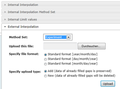
External interpolation
The section "External Interpolation" offers the possibility to conduct an interpolation out of the OBIS and upload the file into OBIS. If you use an external method you need to chose the method in the selection menue or describe a new method. The import function takes only those values which lie within a previously described data gap, even if the timeseries is longer. The values within the data gap were treated by OBIS like interpolated values. The gap interval can only be filled completely or not. If only one value in the timeseries is missing, it will not be used to close the gap.
Further you need to specify the upload file. You can chose add to complement the timeseries or new to add new data after you have previously deleted already exitsing data. This feature allows to close still existing gaps without losing former interpolation results.
Create input files for JAMS
Time series data stored in the database can be used as input data for the Jena Adaptable Modelling System (JAMS). You have the possibility to create a XML-file, which can be used for a direct access from JAMS during a model run, or download an input file for JAMS. An XML file is an Extensible Markup Language file. For more information about JAMS, have a look to the tutorial Applying the J2000 model. You can find the function in the menu 'Time series data' as subitem 'Jams XML'.
By clicking the button "Jams XML" a new screen appears. You need to select a catchment and one parameter. For both you have a pull down menu showing all available catchments and parameters. When you have finished the selection, click on the button "Start".
A list of all entries appears. You can reduce the results by setting a time interval for the time series data. After selecting a time interval, click the button "Set" to store the entries. An updated table of available time series data appears. You can select the data you are interested in by ticking the checkbox. You have also the possibility to view metadata and time series data of the listed datasets by clicking "show" in the respective columns. In the section 5. you will be asked to insert an EPSG/SRID code for the target spatial reference system of the JAMS file. In the section 6. you have to define an identification of missing values. By default this value is set to -9999. In section 7a. you have to name the file. Then you can chose whether you want to "create XML File" or "Download JAMS input file". Note: Do not forget to tick the checkbox of at least one time series of the list!
Indicator calculation
The OBIS offers a function to calculate various indicators within the database. You can access this feature with the subitem "Indicator calc." under the section "Time series data".
By clicking the button "Indicator calc." a new screen appears. You need to select a catchment and one parameter. For both you have a pull down menu showing all available catchments and parameters. When you have finished the selection, click on the button "Start".
You will be asked to set a time period. Otherwise calculation can't take place. You can search for stations fulfilling different attributes. Next to the time period, these are
- kind of year (calendar year, hydrological year)
- show time series with gaps or without gaps
- dsitance of stations to selecetd catchment
- elevation of station
You can select the data you are interested in by ticking the checkbox. You have also the possibility to view metadata and time series data of the listed datasets by clicking "show" in the respective columns.
Note: Do not forget to tick the checkbox of at least one time series of the list! Finally, click on "start indicator calculation". An overview of the indicator calculation appears. For the example "precipittaion" following parameters will be calculated:
- Mean annual precipitation
- Mean annual areal precipitation
- Min
- Mean
- Max
- Standard deviation
- Trend/ Noise
- Term for linear trend: y= bx + a
Further, a plot of the time series is shown provided with an average line and the trendline.


