Model output

Revision as of 09:44, 5 October 2012

The model results and efficiency are provided in three different ways:

• Graphical display
• Numerical output
• Efficiency measurement

Graphical display

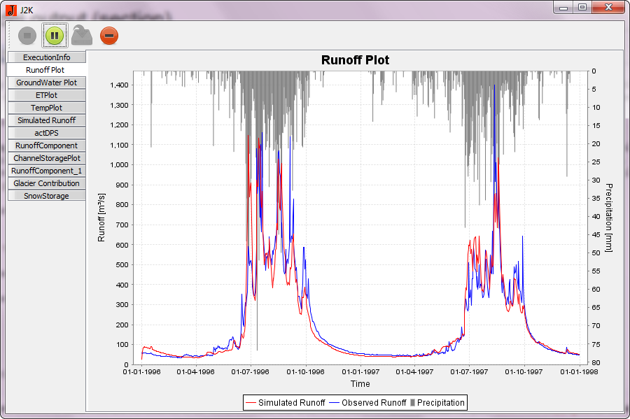
The model provides the graphical display output for many variables. As an example, the output of simulated runoff plot is provided below:

• An example of runoff Plot

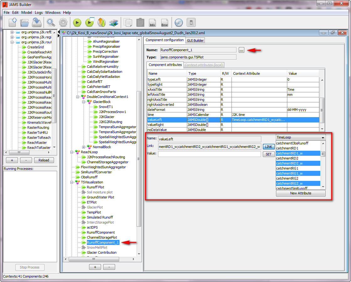
The 'TSVisualization' component of the JAMS builder brings graphical display of different output variables. The 'TSVisualization' component can be expanded (click + and - sign on the left side to expand and reduce) as shown in Figure below. The existing TS plots will be shown. The new plot can be created by using the existing plot. Drag one of the existing plots (example, Glacier contribution) and hold CTRL key (a + sign will appear) and leave both the keys. The new plot will appear with the new name (Glacier contribution_1). From the right window, the name and the values of the new plot can be changed. Mainly, four things has to be changed for the new plot.

1. Change the name of the component. Click the [...] box on the right hand side of the 'Name'. This will bring a new window and you can change the name of the new plot.

2. Provide new names for the legend used in the plot. Click on the 'titleLeft' row and change the name of the legends under 'Value' window. In case of more than one legend, seperate the name by semicolon.

3. Provide colors to the legends. Click 'colorLeft' row and change the color name under 'Value' window.

4. Provide value for the legends. When 'valueLeft' row is clicked, the window below is activated. The value can be choosen from Timeloop. Use CTRL key to choose more than one value.

Alternatively, this information can be changed by editing the model xml file which has been explained below.

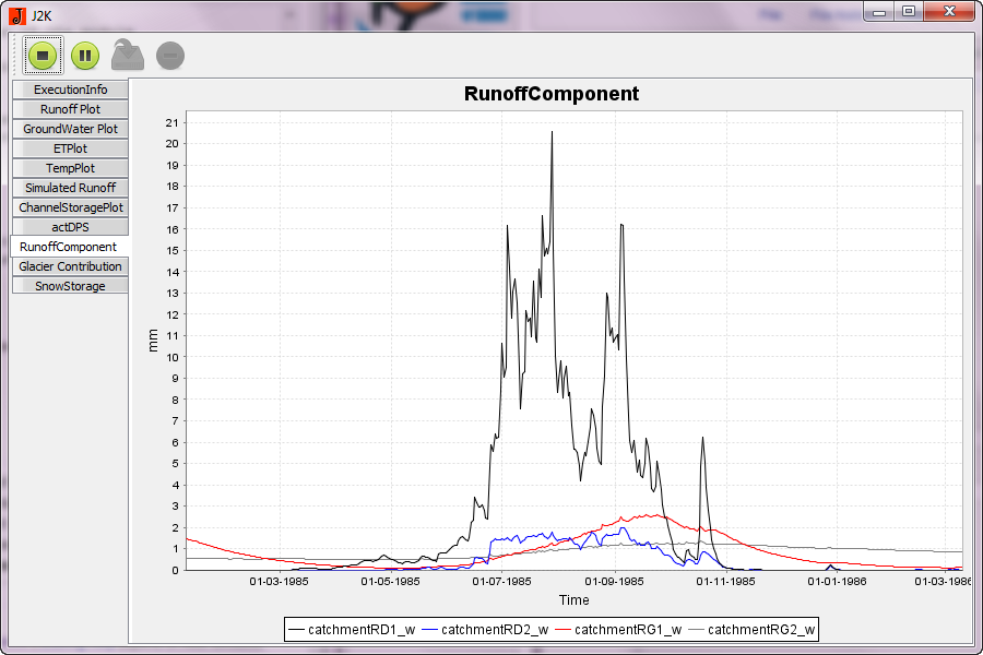
With these lines in xml file as shown in figure below, users can define which output files they wish to see as a plot/graph. In the figure below, four different runoff components is displayed.

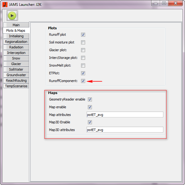
After defining the plot, users also need to define a line in a 'Plot & Maps' component of the xml to bring it in the JAMS framework. This has to be done by directly editing the model xml. For example: The lastline is dedicated to display the Runoff component plot.

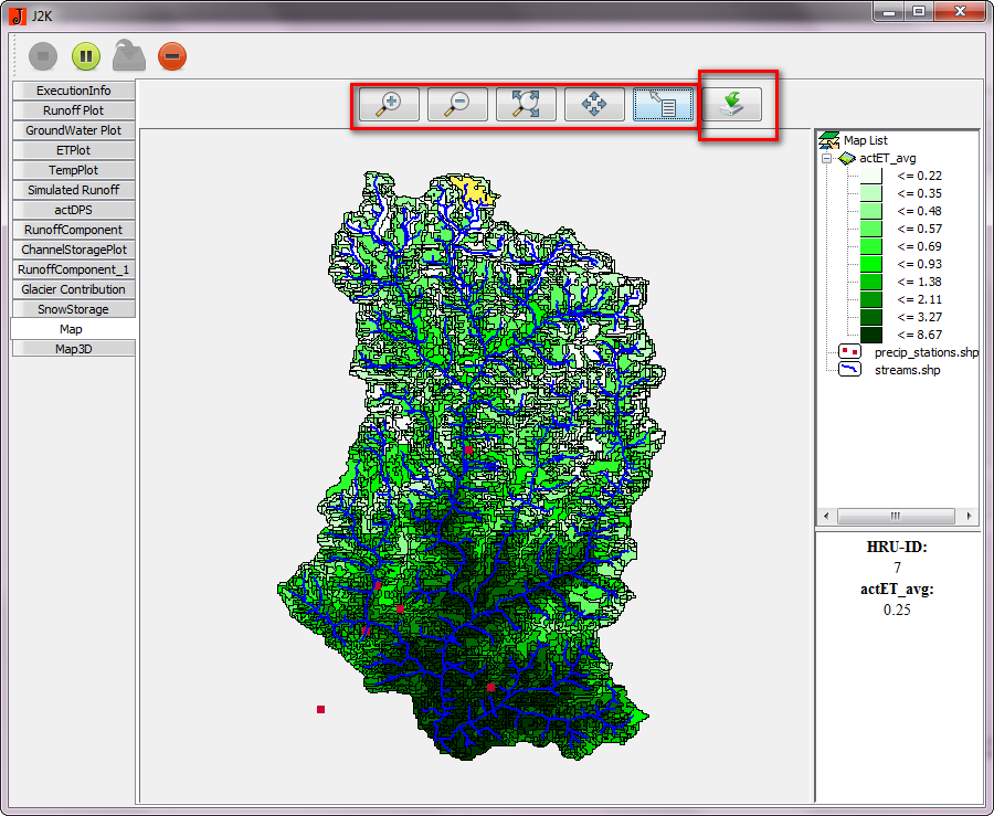
The Runoff component Plot will appear in 'Plots & Maps' group in the JAMS launcher after loading the xml file in JAMS, which users can switch on/off to display as a graph. The spatial distribution of some variables can also be dispaled as a map, for which the different component of 'Maps' (as shown in rectangular red window) has to be activated as shown in Figure below. In this example, the average evapotranspiration of the model run period is activated.

After running the model, users can see the plot of different variables as provided below:

• Runoff component components

• Spatial distribution of evapotranspiration

The values are provided in daily average. Users can zoom in and out the map. Similaly, the values can be downloaded by clicking the save botton (the red box in right hand side). The GIS shape file with HRU ID and values associated with each HRUs are saved.

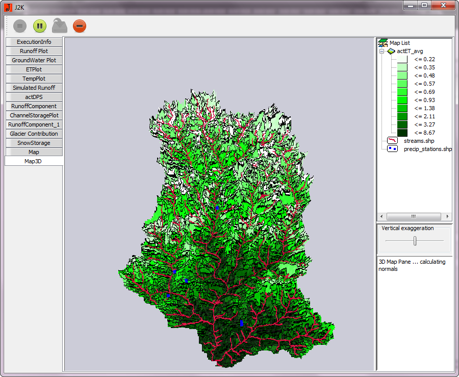
To display the spatial distribution of evapotranspiration in 3D map, users have to click the 'Map 3D'.

Numerical output

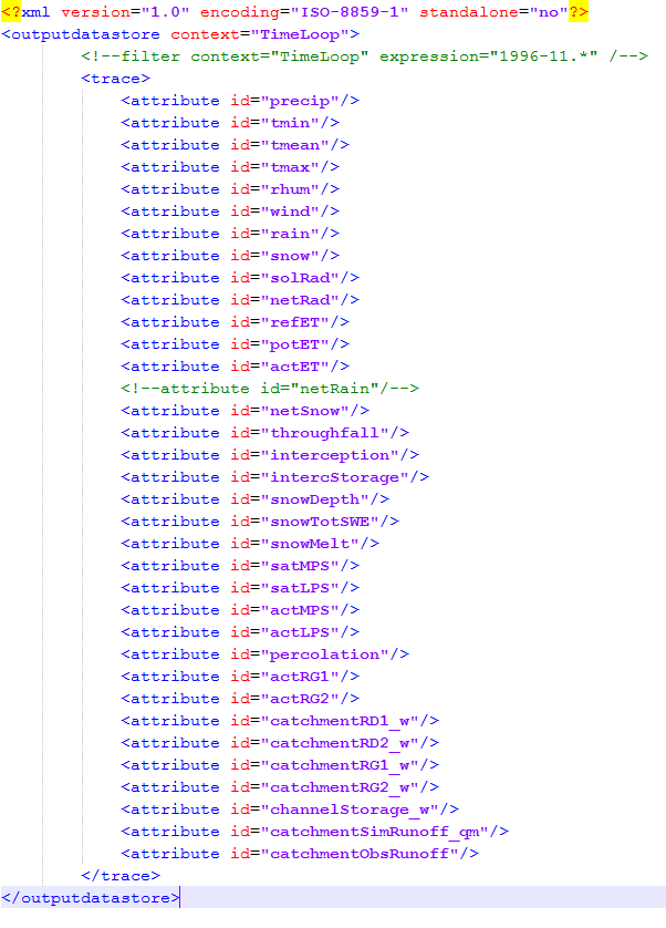
The model outputs on a daily resolution are provided in the output folder (current-->> Timeloop.dat filename) after each model run. The variables which need to be produced as output data is deterimed inside the TimeLoop.xml file which is placed outside the current folder.

The TimeLoop.xml has daily output variables as shown in Figure below. If users do not need some variables, they can comment out the particular variables as shown in the case of netRain in the figure.

• TimeLoop.xml file

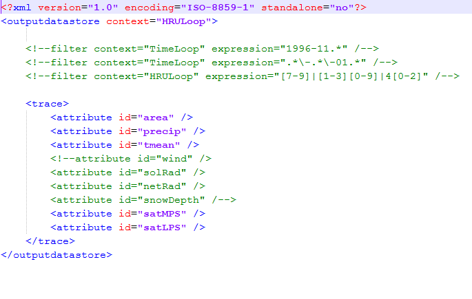
The HRULoop.xml is responsible for producing the daily average values of each variables of interest (as defined inside the xml file) for all HRUs. Users can comment out some variables as shown in the case of wind below.

• HRULoop.xml file

Please note that the HRULoop produces a file which is large in size (due to the information associated all HRUs at each time step). Therefore, it is advised not to produce HRULoop.dat everytime when the model is run. Removing the HRULoop.xml file (from output folder) will not produce HRULoop.dat file.

Efficiency measurement

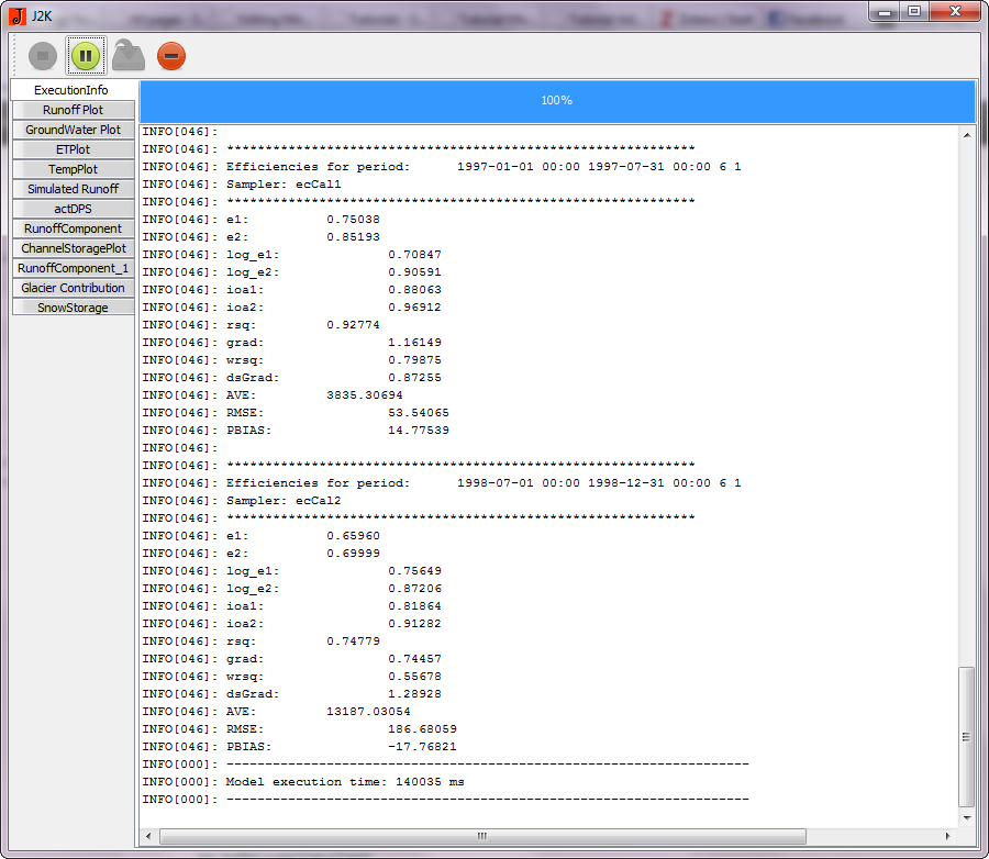
The model produces different efficiency results at the end of each model run. The results are published at the bottom of 'ExicutionInfo' of the JAMS launcher. The model is able to break the time period (such as calibration and validation) into different periods as defined by users.

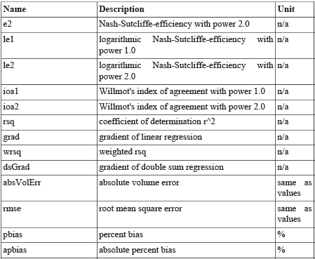
The details of the objective functions are provided below:

To understand more about the objectives function and their pros and cons in terms of simulating different parts of hydrological dynamics, the article (Krause, 2005) might be helpful:

Krause, P., Boyle, D.P., Bäse, F., 2005. Comparison of different efficiency criteria for hydrological model assessment. Advances in Geosciences 31, 89–97.