This documentation aims to guide you through the individual steps of analysing CORDEX datasets with the CDITool. CDITool is a desktop Java App that implements a flexible and user-oriented data analysis workflow that covers the following functions:
- Extraction of precipitation and temperature data of NetCDF model outputs from the Coordinated Regional Climate Downscaling Experiment (CORDEX)
- Calculation of climate indices defined by the Expert Team on Sector-Specific Climate Indices (ET-SCI) based on the extracted data
- Result analysis, visualization and output
CDITool is built on top of the JAMS modelling platform http://jams.uni-jena.de and can easily adapted or extended. It is based on and distributed as Open-Source Software under the GNU Lesser General Public License (LGPL3).
1. Preparation and start
CDITool comes as a ZIP archive that includes all the required files for running the software. The most current version of the software can be downloaded from http://jams.uni-jena.de/cditool. Since it is a Java application, CDITool requires a Java Runtime Environment (JRE) that is packaged in the archive. To run the software, follow these steps:
- Extract the ZIP archive into a new folder
- Start the cditool.exe file in the root of the folder
An empty CDITool window will open in result (Figure 1). If required, the version of the software can be accessed by selecting Help → About from the main menu.

2. Create/open workspace
To start a new data analysis, a workspace has to be created. This is a folder in the file system that contains all the data and files of a single index calculation. To create a new workspace, follow these steps:
- Select File → New Analysis from the menu or press the respective icon in the toolbar
- In the Open dialog, select an existing, empty folder or type the name of a non-existing folder
- Press the Open button
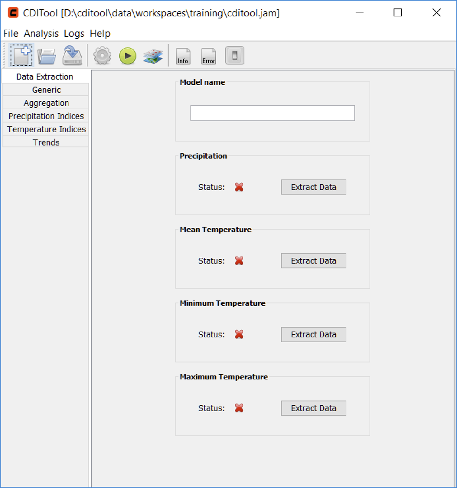
In result, the CDITool window will create the new workspace in the desired location and will open the new analysis view (Figure 2). Each analysis view is separated into panels (shown as tabs) that cover the following functions and settings:
- Data Extraction: functions for selecting the climate model, defining the grid cells to be analyzed and for extracting the related data
- Generic: generic settings of the climate data analysis, covering the analysis period and the core input data to be analyzed
- Aggregation: time intervals for which the input parameters and indices will be aggregated
- Precipitation Indices: selection of / settings for indices based on precipitation
- Temperature Indices: selection of / settings for indices based on temperature
- Trends: selection of / settings for trend calculations
The following sections will explain the available options in more detail.
3. Data extraction from climate models
The first step of calculating climate indices from climate models is the definition of the models’ grid cells to be analyzed and the extraction of the related data. Four datasets have to be processed, including precipitation, mean temperature, minimum temperature, and maximum temperature data. Each of these datasets is processed at a time and has to be provided by a NetCDF dataset that covers the full time period to be analyzed.
The Data Extraction panel shows a list of the four datasets together with an indicator icon showing whether the dataset was extracted already (green check mark) or not (red cross mark) (Figure 2).
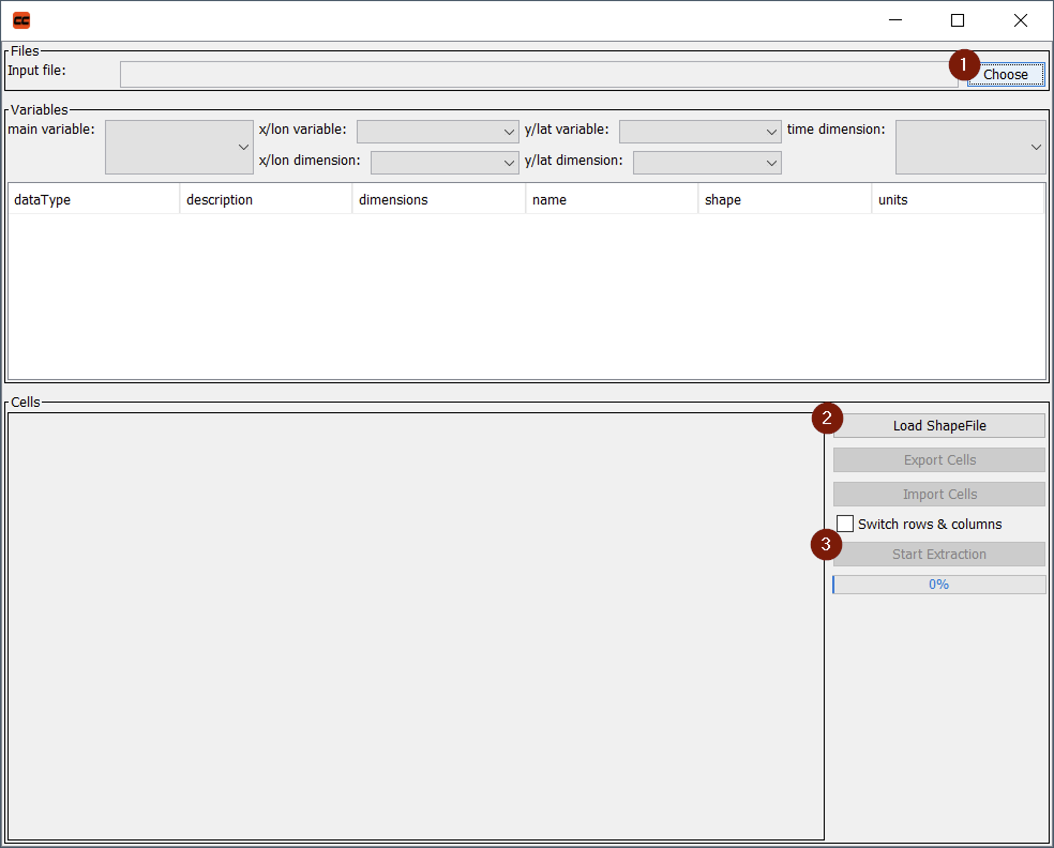
To start the extraction process for one of the datasets, e.g. precipitation, the related Extract Data button has to be pressed. In result, a new window will open (Figure 3). The data extraction procedure consists of three steps with the related buttons marked in Figure 3:
- Selection of a NetCDF input file
- Selection of model grid cells to be analyzed by means of a polygon Shapefile containing the larger region of interest
- Extraction of data
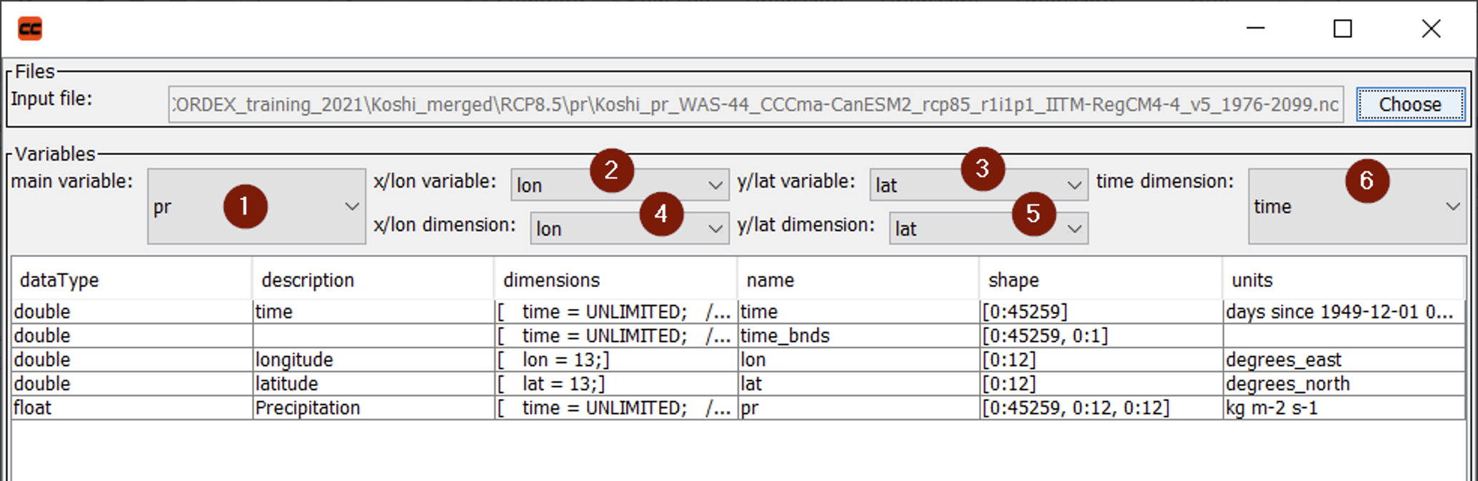
After button 1 was pressed, a file input dialog will ask for the NetCDF input file. After the file was chosen, meta-information is extracted and shown in the upper part of the window (Figure 4). The following NetCDF variables, which are marked in Figure 4, need to be defined:
- the main variable (e.g. precipitation)
- the longitude variable
- the latitude variable
- the longitude dimension variable (differs from #2 for rotated datasets)
- the latitude dimension variable (differs from #3 for rotated datasets)
- the time dimension variable
By default, the software will try to detect this information automatically. However, the identified values should be double-checked to avoid erroneous data. A table below the variable selection will further list meta-information extracted from the NetCDF file.
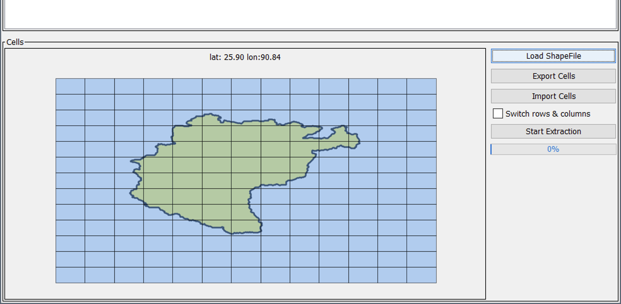
In the next step, the desired model grid cells must be selected. For this purpose, button 2 (Figure 3) is pressed and a polygon Shapefile with the larger region of interest has to be selected. This Shapefile has to intersect the model domain to obtain meaningful results. After the selection of the Shapefile, the contained polygons are displayed in a map view together with the boundaries of all model grid cells (Figure 5).
The map view features basic functions for panning (hold right mouse button), zooming (mouse wheel) and selection of grid cells (left mouse button). After panning/zooming to the area of interest, model grid cells can be selected. This can be done via the following options:
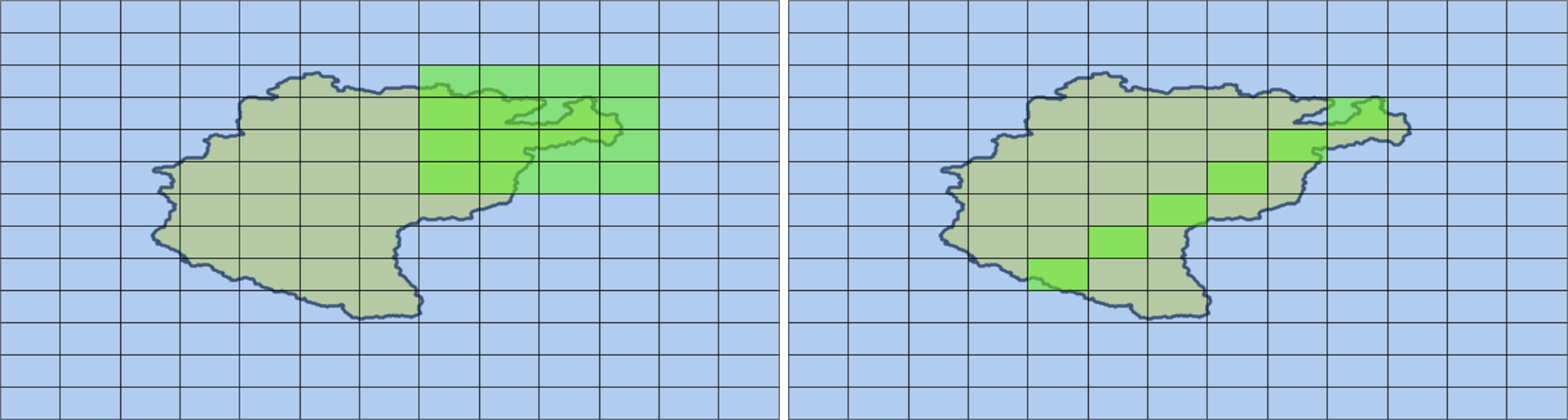
- A rectangular extent can be selected by left-clicking/holding at the upper/left cell, moving the mouse to the lower right cell and releasing the button (Figure 6, left)
- Individual cells can be selected by left-clicking to a first cell, pressing the CTRL-key and subsequently selecting further cells by left-clicking them (Figure 6, right)
After the grid cells have been selected, further, optional functions can be applied (Figure 5, right). A function for exporting and importing of a grid cells selection allows to store the current selection to a text file and to load this selection at a later time. The buttons labelled Export Cells and Import Cells will open related file save/open dialogs that will ask for user defined file name.
Another function allows to switch the orientation of rows and columns (i.e. latitude and longitude) in the NetCDF data file. While this should not be required for standard NetCDF data files, this function may be handy in situations where both dimensions have been changed due to a reprojection of the original data without adapting the NetCDF metadata. In these cases, the checkbox labelled Switch rows & columns can be enabled to ensure correct data extraction.
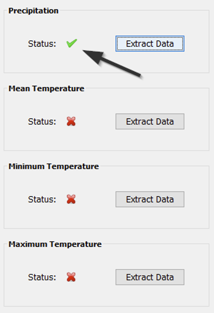
After all settings have been made, the data extraction process can finally be started by pressing the Start Extraction button (Figure 3, button 3). This will extract time series of the selected parameter (e.g. precipitation) for the selected grid cells into a pre-defined text file inside the current workspace. In addition, a Shapefile containing the outline polygons of all selected grid cells will be generated and stored inside the workspace. If the extraction was successful, the status label next to the corresponding dataset in the Data Extraction panel of the CDITool main window will show a green check mark (Figure 7).
This data extraction procedure has to be applied for all required datasets, i.e. precipitation, mean temperature, minimum temperature, and maximum temperature. While the NetCDF input file has to be changed according to the required data, the selected grid cells must stay untouched in order to ensure that all four datasets have been extracted for identical grid cells. At the same time, it must be ensured that NetCDF input files cover the same time period and contain identical spatial and temporal resolutions, i.e. result from the same climate model.
In the case that only the mean temperature of a climate model is available, identical temperature data can be used to provide all three temperature input datasets as a workaround. However, some of the calculated indices will not gain meaningful results. For example, the index DTR (Daily Temperature Range) will only contain zero values since minimum and maximum temperature show identical values. In general, index calculation will not be possible before all four datasets have been provided, i.e. showing four green checkmark icons.
In a final step of the data extraction process, a model name can be provided in the Model name text field of the Data Extraction panel (Figure 2). This model name will be used during the following output of analysis results and will allow to easily compare the indices of different climate models.
4. Index calculation settings
Once all input parameters have been extracted, the software is ready to start the index calculation using recommended settings. However, depending on individual requirements these settings that can be changed. As outlined in section 2.2, the settings are subdivided into five groups, i.e. Generic, Aggregation, Precipitation Indices, Temperature Indices, and Trends which are organized in individual panels/tabs.
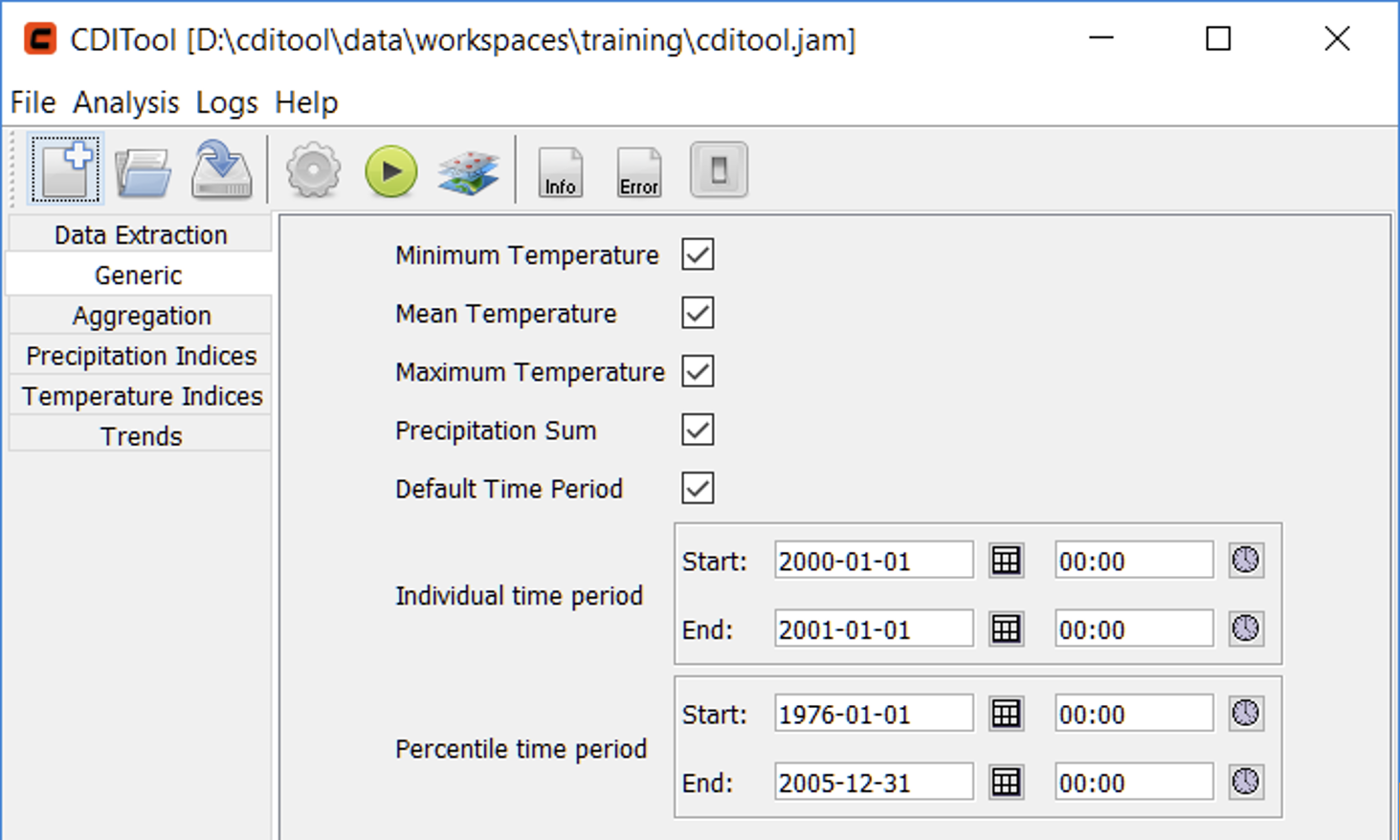
The Generic panel (Figure 8) provides options to enable/disable the aggregation and output of the input variables. Further, the group provides an option to calculate indices only for a user-defined time interval. The latter will be done for the Individual Time Period setting once the check box Default Time Period was disabled. The Percentile Time Period setting defines the time period which will be used for calculating percentile-based indices.
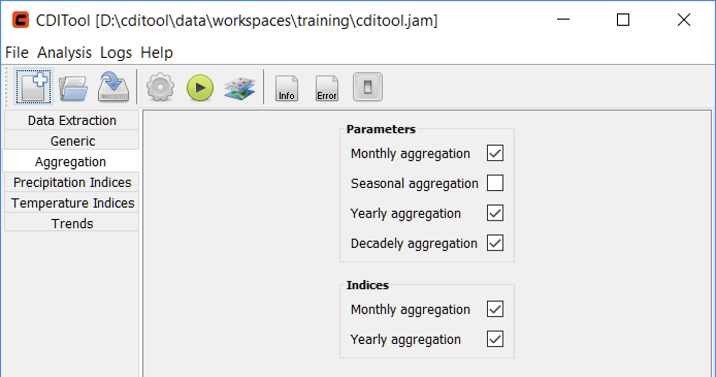
The Aggregation panel (Figure 9) offers options to enable or disable individual aggregation intervals for climate parameters and indices. Disabling any of these options will result in not aggregating indices for the related time periods, which can save processing time and storage space especially for large datasets.
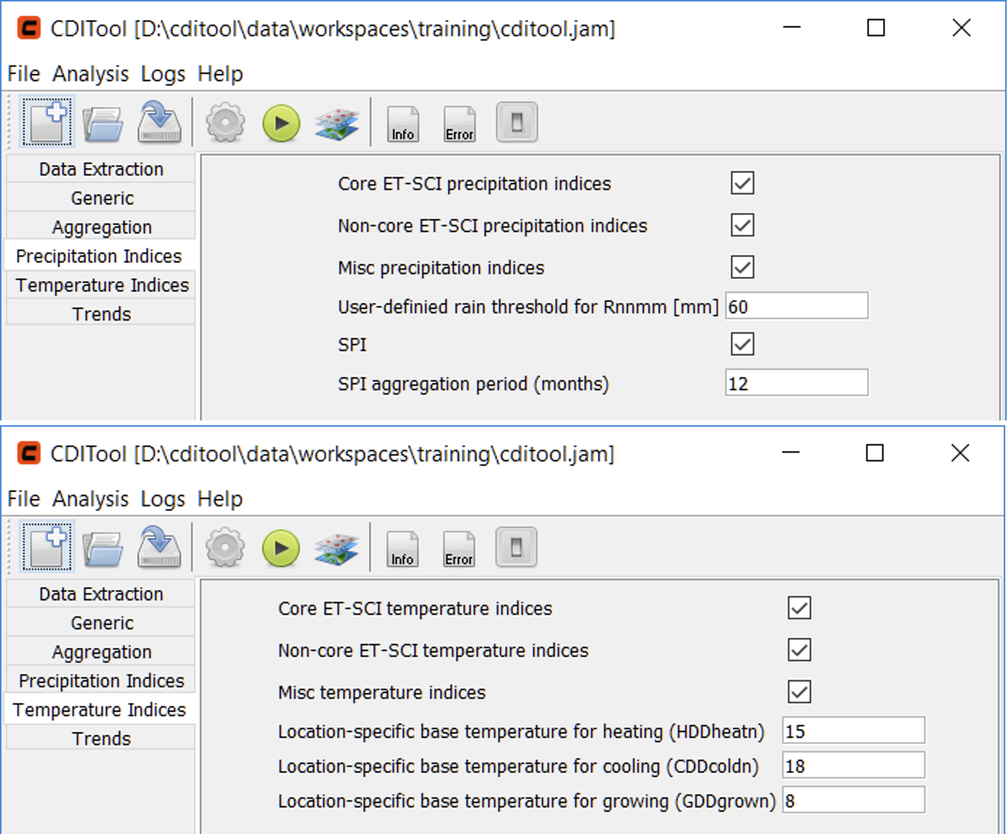
The Precipitation Indices and Temperature Indices panel list options related to the calculation of precipitation and temperature indices (Figure 10). Both panels show three options that allow choosing the extend of indices calculated. These are arranged into the following groups (see appendix):
- Core ET-SCI indices
- Non-Core ET-SCI indices
- Miscellaneous, non-ET-SCI indices
As with aggregation options, disabling any of these options will save processing time and storage space.
In addition, these panels contain index-specific options, such as the rain threshold required for calculating the Rnnmm precipitation index and other user-defined thresholds.
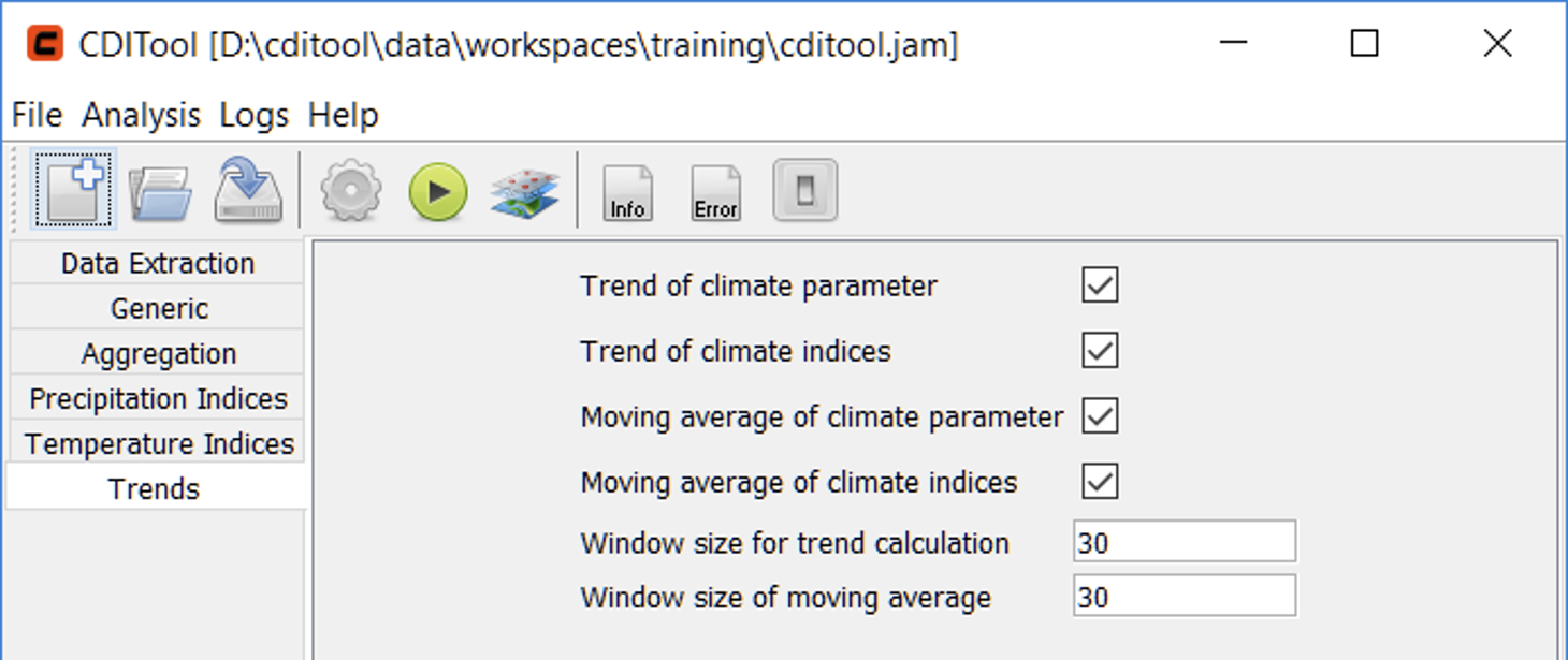
The last panel is related to Trend calculation (Figure 11) and offers options to enable/disable the calculation of trends and moving averages as well as their related window sizes in number of years.
5. Index calculation
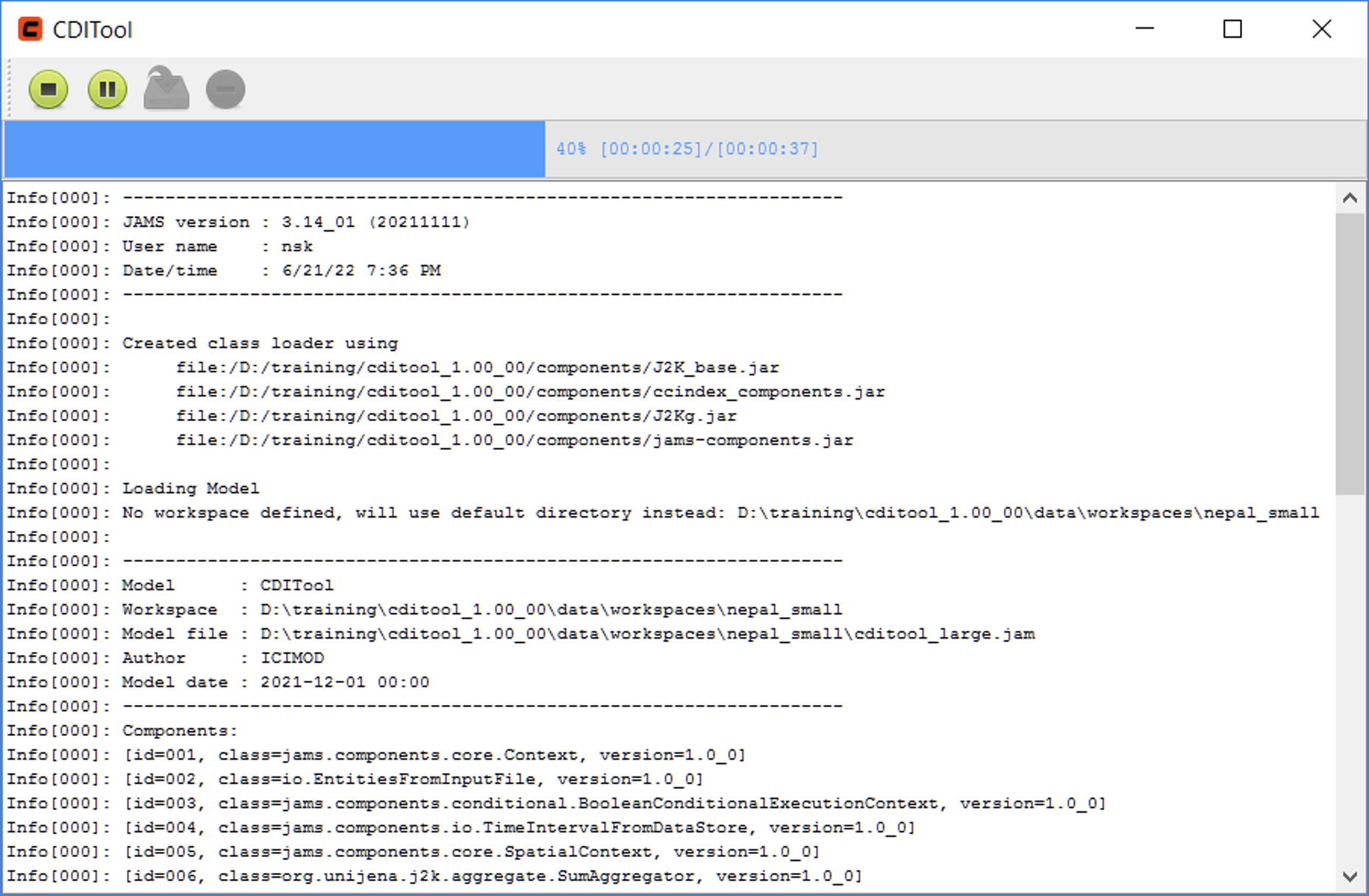
After all required input data have been extracted and settings been made, the actual trend calculation can be started. This is done by pressing the green start button in the tool bar or by choosing Analysis → Start Analysis from the main menu. In result, a window will open that shows the progress of the index calculation and various status outputs (Figure 12). Using the stop button in the tool bar of this window, the index calculation can be stopped. The calculation process is finished once the close button on the right is enabled. Once the calculation is finished, the window can be closed. Closing the window will also end any running index calculation.
6. Result analysis and visualization
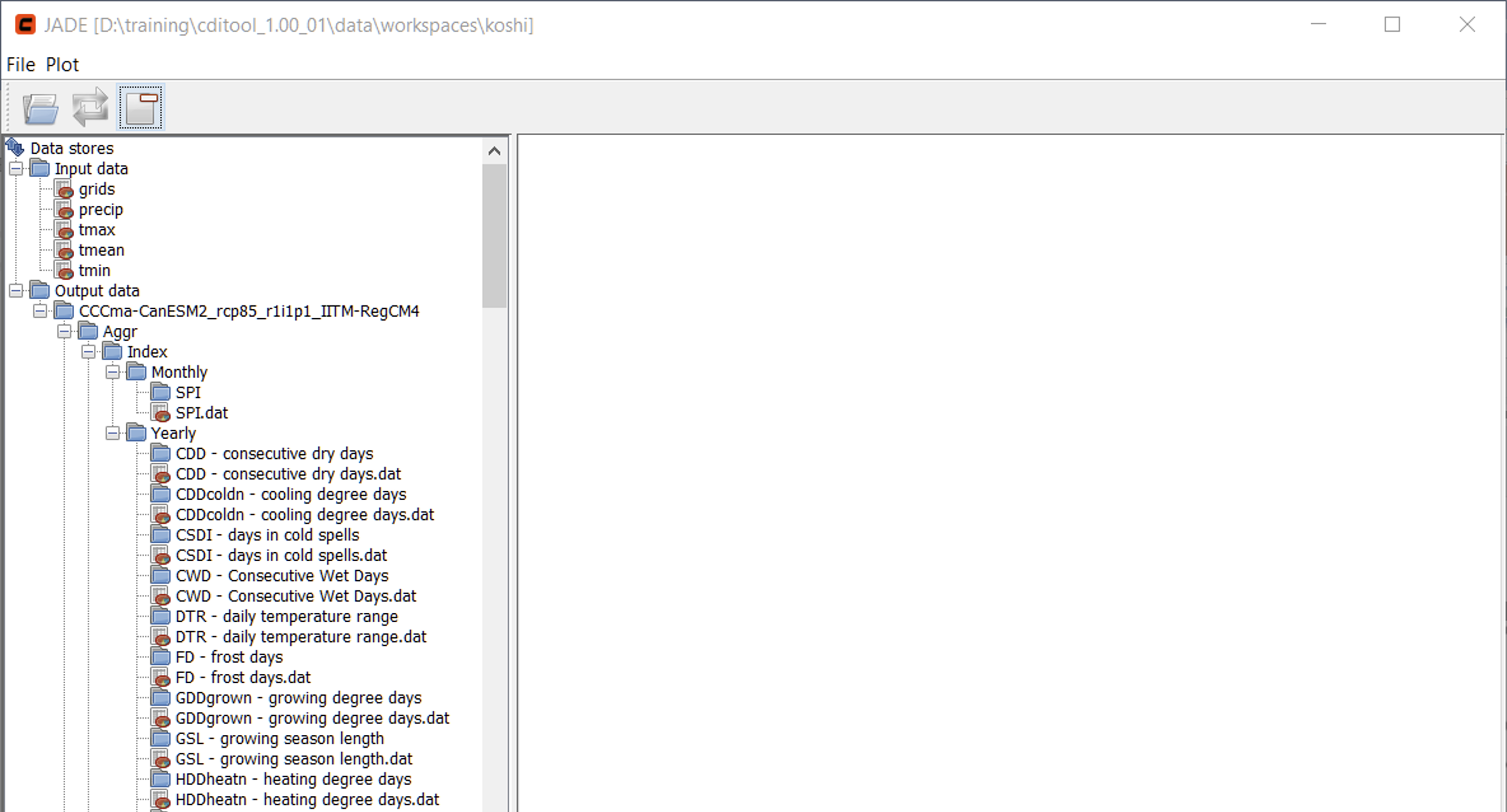
Once the index calculation is finished, its results can be explored by means of the CDITool data explorer (JADE). This separate tool can be opened by pressing the respective data analysis button in the toolbar or by selecting Analysis → Data Explorer from the main menu. Figure 13 shows the start view of JADE.
JADE is separated into two main panels. The panel on the left-hand side shows a tree view that reflects the organization of input and output data files of the workspace. While the input data consist of a single dataset each, all output data come in two flavors:
- As an ASCII file that contains the spatio-temporal result datasets, indicated by a file icon.
- As a Shapefile vector dataset that contains the boundaries of the selected grid cells as geometries and the calculated indices as attribute data of these geometries, indicated by a directory icon.
The panel on the right-hand side shows the content of one or more data files that have been previously selected. Selection of a dataset can be done by double-clicking the respective entry or by right-clicking it and choosing Show data. Shapefiles cannot be analyzed with JADE and have to be further processed in standard GIS software such as QGIS[3].
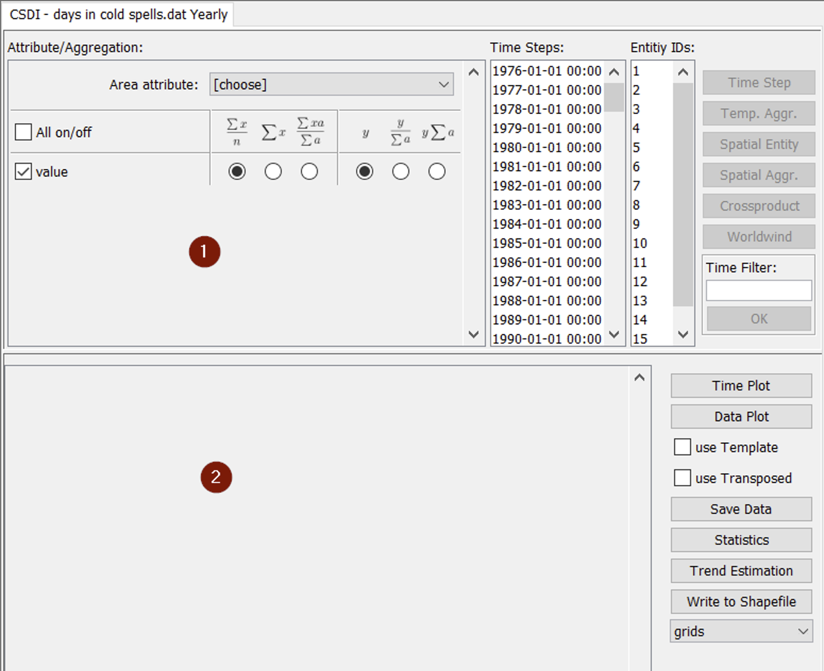
Once a dataset is opened in JADE, a new tabulator panel will open in the right-hand side of the window. While the number of open datasets is not limited, they can be closed by clicking the close button in the tool bar. The dataset view (Figure 14) is again separated into two areas. The upper panel (1) shows the available data, time steps and grid cells of a dataset. The lower panel (2) shows a table view of these data. The way of how the data are transferred into the table view is defined by the user. Here, JADE offers various functions for aggregating the data in time or space and for outputting selected values as a cross-product. Typical use-cases are:
- Show time series of the mean value of all grid cells (spatial aggregation)
- Show the temporal mean across all/selected time steps for all grid cells (temporal aggregation)
- Show time series of a single/multiple grid cells (cross-products)
The following section will give an overview of these options.
6.1 Data aggregation
Spatial aggregation
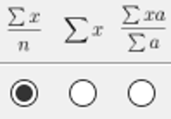
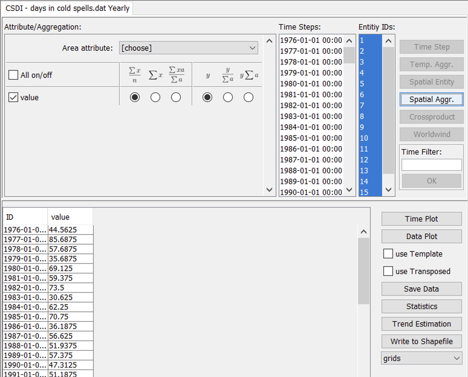
The spatial aggregation requires the selection of the grid cells to be aggregated. This happens by selecting entries from the Entity IDs list. A double click into the list will select all grid cells. This can also be achieved by pressing the CTRL-A key combination. Holding the CTRL-key while left-clicking entries from the list will select arbitrary subsets. Left-clicking a first entry and subsequently left-clicking a second entry while holding the SHIFT-key will select all entries in-between. Once the grid cells have been selected, the type of aggregation must be chosen. Figure 15 shows the three available options: (i) mean, (ii) sum, and (iii) area-weighted mean. Since all grid cells cover the same area, the last option is not needed. In order to choose mean or sum aggregation, select the radio button under your preferred option. To finally calculate the aggregates, press the Spatial Aggr. button. In result, the table in the lower part of the panel will be filled with a time series of the aggregated values. Figure 16 shows the result of a spatial mean of the CSDI over all grid cells.
Temporal aggregation
Temporal aggregation is very similar to spatial aggregation with the difference that date entries from the Time Steps list are chosen this time. The selection of date entries follows the same procedure as with the selection of grid cells. The same applies for the configuration of the aggregation type (sum vs. mean). The calculation the aggregates is triggered by pressing the Temp. Aggr. button this time. In result, the table in the lower part of the panel will be filled with a list of aggregated values for each grid cell.
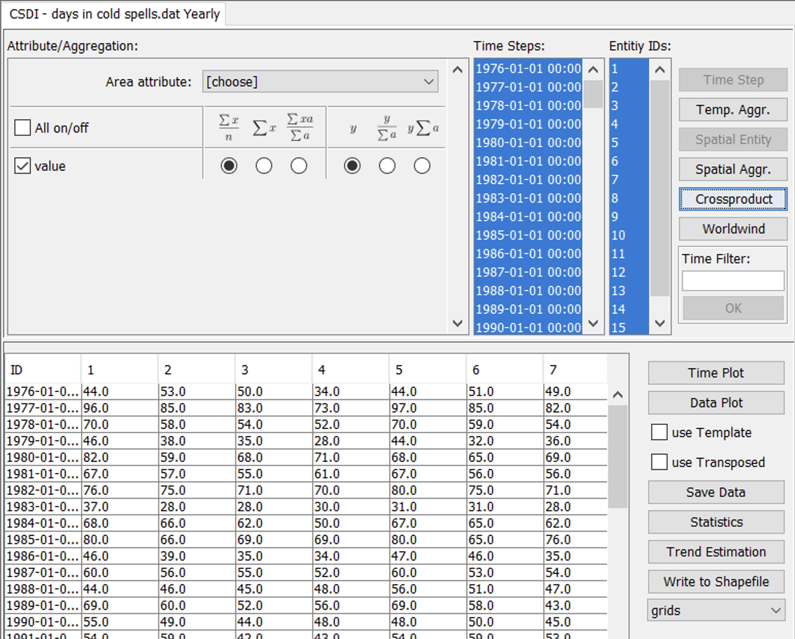
Cross-products
The cross-product output option simply extracts the data for all selected dates and grid cells as a table. Alternatively, the data can directly be transferred into the integrated Worldwind viewer for further exploration (see section 2.6.2 Worldwind). Figure 17 shows an example result of the cross-product output option.
6.2 Data visualization
Charts
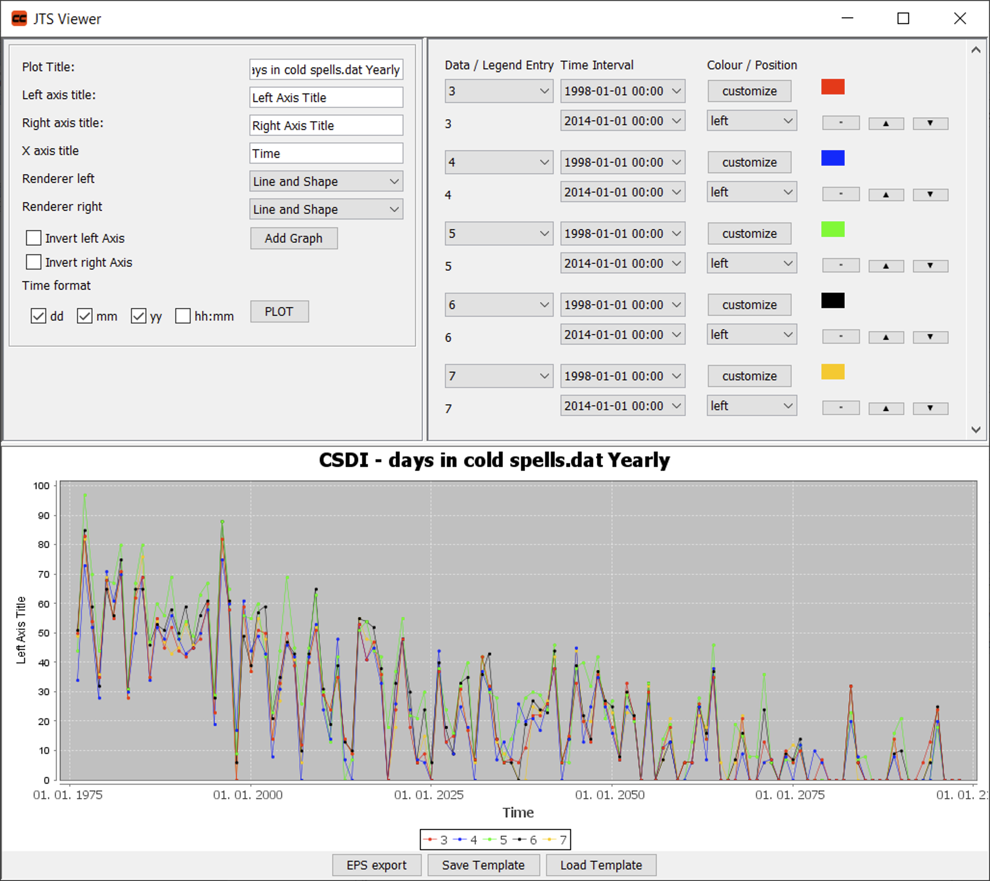
The easiest way of visualizing tabular data is by using charts. Once data are listed in the table view of the lower panel, they can be visualized by means of time plots (first column contains dates) or data plots. This is done by selecting the data that should be visualized (key combo CTRL-A will select all data) and subsequently pressing the Time Plot or Data Plot buttons. Figure 18 shows an example of a time series visualization using five grid cells. The charts offer zoom functionality (drag & drop inside the plot area), image output functions (right click inside the plot area). A variety of options within the plot viewer allows to further tune the layout of the plot.
Worldwind
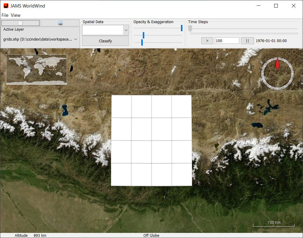
Visualization of spatio-temporal data is supported by means of the build-in Worldwind[4] viewer. For this to work, dates and grid cells of interest have to be selected first, such as for the Cross-product output. Afterwards, the Worldwind button must be pressed. In result, the Worldwind viewer will open and zoom to the location of the selected grid cells (Figure 19). In a next step, the data must first be classified in order to visualize them. This is initiated by pressing the Classify button. Another window will open, offering options for data classification. These include the number of classes and the classification method. Pressing the Calculate button will initiate the classification of the data and will show a histogram of the data distribution. The color setting will further allow to select a start color (linked to the first class) and an end color (linked to the last class). Once the colors have been selected, the classification settings can be applied to the visualization by pressing the Apply button.
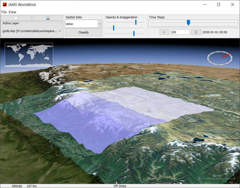
Once the classification was applied, the view port of the Worldwind viewer can be changed by right-clicking inside the map while moving the mouse. At the same time, the mouse wheel can be used to zoom in or out. To change the display date, the Time Steps slider can be used to move forward/backward in time. The play button below the Time Steps slider can further be pressed to automatically change to the next date after a defined number of milliseconds. The latter can be adjusted by means of a text field next to the play button. Detail information about the data of a single grid cell can be accessed by left-clicking into the grid cell. Figure 20 shows an example output of the Worldwind viewer.