Water and Nutrient Balance Model J2000-S
(→Dynamik der Residuenpools) |
(→Dynamics of the Residua Pools) |
||
| Line 313: | Line 313: | ||
The transfer rate is substracted from the active pool whereas it is added to the nitrate pool. | The transfer rate is substracted from the active pool whereas it is added to the nitrate pool. | ||
| − | ====Dynamics of the | + | ====Dynamics of the Residue Pools==== |
| − | The dynamics of the decomposition of fresh organic substances ( | + | The dynamics of the decomposition of fresh organic substances (residue) from plant remains and organic fertilizer is carried out only in the top horizon. the residue are divided in two pools: the first one represents the biomass as a whole, the second represents the residue's amount of nitrogen. The supply to the residue pools is carried out via plant remains after the harvest and via the organic fertilization with the help of the following equation: |
<math>Residue_{pool} = Residue_{pool} + inp_{biomass} + (fertorgN_{fresh} \cdot 10)\! </math> | <math>Residue_{pool} = Residue_{pool} + inp_{biomass} + (fertorgN_{fresh} \cdot 10)\! </math> | ||
| Line 323: | Line 323: | ||
with | with | ||
| − | '' <math>Residue_{pool}\!</math> = | + | '' <math>Residue_{pool}\!</math> = residue pool [kg/ha]'' |
'' <math>inp_{biomass}\!</math> = input biomass [kg/ha]'' | '' <math>inp_{biomass}\!</math> = input biomass [kg/ha]'' | ||
| Line 329: | Line 329: | ||
'' <math>fertorgN_{fresh}\!</math> = input nitrogen via organic fertilization [kgN/ha]'' | '' <math>fertorgN_{fresh}\!</math> = input nitrogen via organic fertilization [kgN/ha]'' | ||
| − | '' <math>N_{residue_{pool}}\!</math> = | + | '' <math>N_{residue_{pool}}\!</math> = residue pool's amount of nitrogen [kgN/ha]'' |
| − | The decomposition of the | + | The decomposition of the residue pool is carried out against the carbon-nitrogen relation (C/N-relation). The calculation of the C/N-relation is carried out according to the following equation. |
<math>\epsilon_{C/N} = \frac{Residue_{pool} \cdot 0.58} {N_{residue_{pool}} + NO_3Pool}</math> | <math>\epsilon_{C/N} = \frac{Residue_{pool} \cdot 0.58} {N_{residue_{pool}} + NO_3Pool}</math> | ||
| Line 348: | Line 348: | ||
'' <math>\epsilon_{C/N}\!</math> = C/N-relation [-]'' | '' <math>\epsilon_{C/N}\!</math> = C/N-relation [-]'' | ||
| − | '' <math>\gamma_{ntr}\!</math> = | + | '' <math>\gamma_{ntr}\!</math> = residue decomposition factor [-]'' |
| − | '' <math>Residue_{pool}\!</math> = | + | '' <math>Residue_{pool}\!</math> = residue pool [kg/ha]'' |
'' <math>NO_3Pool\!</math> = nitrate pool [kgN/ha]'' | '' <math>NO_3Pool\!</math> = nitrate pool [kgN/ha]'' | ||
| − | '' <math>N_{residue_{pool}}\!</math> = | + | '' <math>N_{residue_{pool}}\!</math> = residue pool's amount of nitrogen [kgN/ha]'' |
| − | The decomposition constant of the | + | The decomposition constant of the residue pool is calculated with <math>\gamma_{ntr}</math>, <math>\gamma_{water}</math>, <math>\gamma_{temp}</math>: |
'' <math>\delta_{ntr} = \beta_{rsd} \cdot \gamma_{ntr} \cdot \sqrt{\gamma_{water} \cdot \gamma_{temp}}\!</math> | '' <math>\delta_{ntr} = \beta_{rsd} \cdot \gamma_{ntr} \cdot \sqrt{\gamma_{water} \cdot \gamma_{temp}}\!</math> | ||
| Line 364: | Line 364: | ||
with | with | ||
| − | '' <math>\delta_{ntr}\!</math> = constant | + | '' <math>\delta_{ntr}\!</math> = constant of the redidue decomposition’s rate [-]'' |
| − | '' <math>\gamma_{ntr}\!</math> = | + | '' <math>\gamma_{ntr}\!</math> = residue decomposition factor [-]'' |
| − | '' <math>\beta_{rsd}\!</math> = | + | '' <math>\beta_{rsd}\!</math> = residue decomposition coefficient; default value = 0.05 [-]'' |
'' <math>\gamma_{water}\!</math> = soil humidity coefficient [-]'' | '' <math>\gamma_{water}\!</math> = soil humidity coefficient [-]'' | ||
| Line 374: | Line 374: | ||
'' <math>\gamma_{temp}\!</math> = soil temperature coefficient [-]'' | '' <math>\gamma_{temp}\!</math> = soil temperature coefficient [-]'' | ||
| − | The decomposition of the | + | The decomposition of the residue pools is carried out with the decomposition constant of the residue pool. At this, the nitrogen part is allocated to the active organic pool, in terms of humification, and the nitrate pool, in terms of mineralization, in a ratio of 20%:80%: |
<math>Residue_{pool}2 = Residue_{pool}1 - (\delta_{ntr} \cdot Residue_{pool}1)\!</math> | <math>Residue_{pool}2 = Residue_{pool}1 - (\delta_{ntr} \cdot Residue_{pool}1)\!</math> | ||
| Line 386: | Line 386: | ||
with | with | ||
| − | '' <math>\delta_{ntr}\!</math> = constant | + | '' <math>\delta_{ntr}\!</math> = constant of the redidue decomposition’s rate [-]'' |
| − | '' <math>Residue_{pool}1\!</math> = | + | '' <math>Residue_{pool}1\!</math> = residue pool before the time step [kgN/ha]'' |
| − | '' <math>Residue_{pool}2\!</math> = | + | '' <math>Residue_{pool}2\!</math> = residue pool after the time step [kgN/ha]'' |
'' <math>N_{active_{pool}}1\!</math> = active organic pool before the time step [kgN/ha]'' | '' <math>N_{active_{pool}}1\!</math> = active organic pool before the time step [kgN/ha]'' | ||
| Line 400: | Line 400: | ||
'' <math>NO_3Pool2\!</math> = soil nitrate pool before the time step [kgN/ha]'' | '' <math>NO_3Pool2\!</math> = soil nitrate pool before the time step [kgN/ha]'' | ||
| − | '' <math>N_{residue_{pool}}1\!</math> = amount of nitrogen of the | + | '' <math>N_{residue_{pool}}1\!</math> = amount of nitrogen of the residue pool before the time step [kgN/ha]'' |
| − | '' <math>N_{residue_{pool}}2\!</math> = amount of nitrogen of the | + | '' <math>N_{residue_{pool}}2\!</math> = amount of nitrogen of the residue pool after the time step [kgN/ha]'' |
====Denitrifikation==== | ====Denitrifikation==== | ||
Revision as of 21:47, 9 December 2009
Das Wasser- und Stofftransportmodell J2000-S ermöglicht die Simulation des Wasser- und Stickstoffhaushaltes von Mesoskaligen Einzugsgebieten. Das Modell stellt eine Erweiterung des Modells J2000 dar mit denen es die meisten Komponenten zur Beschreibung des hydrologischen Kreislaufs teilt. Zur Beschreibung des Stickstoffhaushalts werden die zusätzlichen Komponenten Bodentemperatur, Bodenstickstoffhaushalt, Landnutzungsmanagement, Pflanzenwachstum und Grundwasserstickstoffhaushalt beschrieben werden. Weitere Module wurden für die Erfordernisse des Stickstoffhaushalts angepasst.
Contents |
Bodenstickstoffmodul
Die Beschreibung des Bodenstickstoffhaushalts erfolgt analog zu der im Modell SWAT (Arnold et al. 1998). Hierbei werden in den einzelnen Bodenhorizonten die 5 Stickstoffpools für Nitrat, Ammonium, stabile organische Substanz, aktive organische Substanz, frische Pflanzenrest Biomasse unterschieden. Die Flüsse und Transformationen zwischen den Pools und außerhalb des Bodens: Nitrifikation, Denitrifikation, Mineralisation, Volatilation, Pflanzenaufnahme und Auswaschung, werden durch empirische Beziehungen in Abhängigkeit der Bodenfeuchte und Bodentemperatur berechnet. Der Nitratfluss wird äquivalent zum Wassertransport durch ein Routingverfahren zwischen den Teilflächen und zum Vorfluter weitergegeben (vgl. Abbildung 1).
Der Stickstoffeintrag über Düngung und Bestandesabfall wird, ebenso wie der Entzug durch die Pflanzen, vom Pflanzenwachstums- und Landnutzungsmanagementmodul bereitgestellt. Die mineralischen Einträge werden dem Ammoniumpool oder direkt dem Nitratpool zugeführt. Der organische Stickstoff geht entweder in die Pools für den Bestandesabfall oder in den aktiven organischen Pool ein. Der Abbau des Bestandesabfalls geht in Abhängigkeit vom C/N-Verhältnis in Anteilen in den Nitratpool oder in den aktiven organischen Pool ein. Der aktive organische Pool steht im Gleichgewicht mit dem stabilen organischen Pool. Der Nitratpool stellt die zentrale Verteilstelle für die Austräge in Form von Auswaschung, Pflanzenaufnahme und Denitrifikation dar. Die im Modul beschriebenen Prozesse finden in verschiedenen frei parametrisierbaren Bodenhorizonten statt. Hierbei beschränken sich die Zuführung von organischer Substanz und Dünger und die Abfuhr von Stickstoff mit dem Oberflächenabfluss auf den obersten Horizont.
Figure 1: Structure of the soil nitrogen module
The here applied nitrogen module contains some simplifications. Thus, no Pflanzenaufnahme from the ammonium pool is offered. Furthermore, the decomposition of organic substances is directly simulated to nitrate without any detour via ammonium. The N immobilization from mineral to organic nitrogen in the soil zone is neglected completely. The water transport of nitrogen is shown very generalized. Thus, a complete mixing of nitrogen in the individual storages takes place instead of advection and dispersion. The individual processes are described in the model as follows:
Pflanzenaufnahme
At first, the plant’s demands (potential Pflanzenaufnahme) which shall be met by the soil nitrogen storage per day t0 are generated:
 [1]
[1]
with:
 = potential Pflanzenaufnahme [kgN/ha]
 = optimal biomass [kgN/ha]
 = actual biomass [kgN/ha]
Afterwards, the proportions of the soil horizons which lie within the effective root zone are generated. At this, the horizons which lie completely within the root zone are taken into account completely (partroot = 1). However, the horizon which lies only partly in the root zone is only considered partly:
![partroot[i] = \frac {rootdepth - layerdepth[i - 1]}{layerdepth[i] - layerdepth[i - 1]} \!](/ilmswiki/uploads/math/9/4/9/94988578303bd534638cb5e0651802fb.png) [2]
[2]
with:
 = horizon [-]
 = proportion of the horizon at the root zone [-]
 = lower threshold of soil horizon [-]
The allocation of the n-uptake to the individual horizons is carried out against a calibration parameter ( ). At this, the potential uptake for the individual horizons is calculated:
![potNup_z[i] = \frac {potNup} {1 - \exp(-\beta_{Ndist})} \cdot \left(1 - \exp\left(-\beta_{Ndist} * \frac {layerdepth[i]} {rootdepth}\right)\right) - uptake[i-1]](/ilmswiki/uploads/math/3/7/0/3707f7d3586df91bd005046e7176d435.png) [3]
[3]
with:
= Horizont [-]
= proportion of the horizon at the root zone [-]
= lower threshold of the soil horizon [-]
= potential Pflanzenaufnahme [kgN/ha]
 = potential Pflanzenaufnahme in the individual horizons [kgN/ha]
 = potential Pflanzenaufnahme which has been taken from upper horizons already [kgN/ha]
= distribution parameter of the Pflanzenaufnahme; default value = 1.0; possible values 1 - 15 [-]
For the calculation of the potential Pflanzenaufnahme which is covered by upper horizons already, the following connection is applied:
![uptake = uptake + potNup_z[i] \!](/ilmswiki/uploads/math/c/9/7/c9702b635f7c1db449196a0c17994b7a.png) [4]
[4]
= potential Pflanzenaufnahme in the individual horizons [kgN/ha]
= potential Pflanzenaufnahme which has been taken from upper horizons already [kgN/ha]
The calculation of a demand is carried out according to the following equation:
![demand = (NO_3Pool[i] \cdot partroot[i]) - potNup_z[i] \!](/ilmswiki/uploads/math/3/b/e/3beb853670497bc45c37498ec5baed42.png) [5]
[5]
with:
= horizon [-]
t = proportion of the horizon of the root zone [-]
 = demand that can be met by the soil nitrogen pool [kgN/ha]
 = soil nitrogen pool [kgN/ha]
= potential Pflanzenaufnahme in the individual horizons [kgN/ha]
If this demand is greater than 0, it can be met by the existing nitrogen storage with:
![NO_3Pool2[i] =
\begin{cases}
NO_3Pool1[i] - potNup_z[i] & \mathrm{f\ddot{u}r} \; \; demand >= 0 \\
NO_3Pool1[i] - (NO_3Pool1[i] \cdot partroot[i])& \mathrm{f\ddot{u}r} \; \; demand < 0
\end{cases}](/ilmswiki/uploads/math/a/3/1/a312b06a7c8f2e01cd7b524cde87eb2b.png)
and
![demand =
\begin{cases}
demand[i] = 0 & \mathrm{f\ddot{u}r}\; \; demand >= 0 \\
demand[i] = demand &\mathrm{f\ddot{u}r} \; \; demand < 0
\end{cases}](/ilmswiki/uploads/math/a/9/2/a92440f6c49c729de089ed8e1ea21283.png)
with
= horizon [-]
= demand that can be met by the soil nitrogen pool [kgN/ha]
 = soil nitrate pool before the time step [kgN/ha]
 = soil nitrate pool after the time step [kgN/ha]
 = potential Pflanzenaufnahme in the individual horizons [kgN/ha]
= proportion of the horizon of the root zone [-]
Anschließend berechnet sich die aktuelle Pflanzenaufnahme aus der potentiellen Pflanzenaufnahme und dem über die Horizonte summierten Bedarf:
![N_{uptake} = potNup + \sum^{n}_{i=1}{demand[i]} \!](/ilmswiki/uploads/math/e/c/d/ecd12f7c1e2fb802760d78eb62419a0b.png) [10]
[10]
with
= horizon [-]
 = proportion of the horizon of the root zone [-]
= demand which can be met by the soil nitrogen pool [kgN/ha]
= potential Pflanzenaufnahme [kgN/ha]
 = actual Pflanzenaufnahme [kgN/ha]
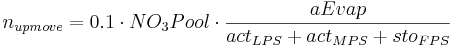
Nitrate Rising by Evaporation
Soil water from deeper layers is transported into upper horizons via the evaporation flux. This happens for each horizon according to the SWAT method:
 [1]
[1]
with
 = amount of nitrogen from the individual horizon which is transported by evaporation [kgN/ha]
= soil nitrogen pool [kgN/ha]
 = actual evapotranspiration of the horizon [l]
 = actual large pore storage of the horizon [l]
= actual middle pore storage of the horizon [l]
 = fine pore storage of the horizon [l]
Transformation Processes in the Soil
Nitrification and Ammonium Volatilation
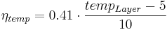
The transformation processes of the ammonium pool in this model are the nitrification from ammonium to nitrate and the ammonium volatilation. The calculation of the total transformation of the ammonium pool is carried out for both processes together. Afterwards, the rates for both processes are separated. In order to represent the influence of the temperature, the following coefficient needs to be calculated:
 [1]
[1]
with
 = soil temperature coefficient [-]
 = temperatur of the soil layer [°C]
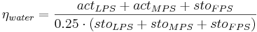
The influence of the soil humidity on the nitrification is described via the coefficient eta_water:
for 
 [2]
[2]
for 
 [3]
[3]
with
 = soil humidity coefficient[-]
 = maximum large pore storage of the horizon [l]
 = maximum middle pore storage of the horizon [l]
= maximum fine pore storage of the horizon [l]
= actual large pore storage of the horizon [l]
 = actual middle pore storage of the horizon [l]
The dependency of the ammonium volatilation on the soil depth is calculated with the following equation:
 = soil depth coefficient [-]
= layer depth of the horizon [cm]
The total Gesamtumsatz of the ammonium pool can be calculated as follows:

This Gesamtumsatz is then distributed into:


with
= soil humidity coefficient [-]
= soil temperature coefficient [-]
= soil depth coefficient [-]
 = soil humidity coefficient [kgN/ha]
 = Gesamtumsatz of the ammonium pool [kgN/ha]
 = fraction nitrification [-]
 = fraction ammonium volatilation [-]
 = amount of nitrifikation [kgN/ha]
 = amount of ammoniumvolatilation [kgN/ha]
Pre-calculation for the Influence of the Environmental Conditions
In order to show the influence of the soil temperature and the soil humidity in the different transformation processes, the following coefficients are calculated beforehand: U
 [1]
[1]
with
 = soil temperature coefficient [-]
= temperature of the soil layer [°C]
 [2]
[2]
with
 = soil humidity coefficient [-]
= maximum large pore storage of the horizon [l]
= maximum middle pore storage of the horizon [l]
= maximum fine pore storage of the horizon [l]
= actual large pore storage of the horizon [l]
= actual middle pore storage of the horizon [l]
Transfer between the Organic Pools
The transfer between the active and the stable organic pool can be calculated with the following equation:

with
 = transfer rate between the active and the stable organic pool [kgN/ha]
 = transfer constant between the active and the stable organic pool; default value= 0.00001 [-]
 = active organic pool [kgN/ha]
 = stable organic pool [kgN/ha]
 = fraction of the organic nitrogen in the active organic pool = 0.02 [-]
The transfer rate is here subtracted from the active pool whereas it is added to the stable pool.
Mineralization of the Active Pool
The active pool is mineralized to nitrate directly without taking the nitrification into account. The rate is calculated as follows:

with
 = transfer rate between the active organic and the nitrate pool [kgN/ha]
 = transfer constant between the active organic and the nitrate pool; default value = 0.002 [-]
= active organic pool [kgN/ha]
= soil humidity coefficient [-]
= soil temperature coefficient [-]
The transfer rate is substracted from the active pool whereas it is added to the nitrate pool.
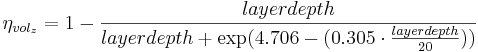
Dynamics of the Residue Pools
The dynamics of the decomposition of fresh organic substances (residue) from plant remains and organic fertilizer is carried out only in the top horizon. the residue are divided in two pools: the first one represents the biomass as a whole, the second represents the residue's amount of nitrogen. The supply to the residue pools is carried out via plant remains after the harvest and via the organic fertilization with the help of the following equation:


with
 = residue pool [kg/ha]
 = input biomass [kg/ha]
 = input nitrogen via organic fertilization [kgN/ha]
 = residue pool's amount of nitrogen [kgN/ha]
The decomposition of the residue pool is carried out against the carbon-nitrogen relation (C/N-relation). The calculation of the C/N-relation is carried out according to the following equation.
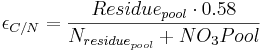
with
 = C/N-relation [-]
 = residue decomposition factor [-]
= residue pool [kg/ha]
= nitrate pool [kgN/ha]
= residue pool's amount of nitrogen [kgN/ha]
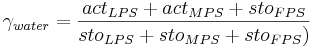
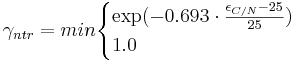
The decomposition constant of the residue pool is calculated with γntr, γwater, γtemp:

with
 = constant of the redidue decomposition’s rate [-]
= residue decomposition factor [-]
 = residue decomposition coefficient; default value = 0.05 [-]
= soil humidity coefficient [-]
= soil temperature coefficient [-]
The decomposition of the residue pools is carried out with the decomposition constant of the residue pool. At this, the nitrogen part is allocated to the active organic pool, in terms of humification, and the nitrate pool, in terms of mineralization, in a ratio of 20%:80%:


with
= constant of the redidue decomposition’s rate [-]
 = residue pool before the time step [kgN/ha]
 = residue pool after the time step [kgN/ha]
 = active organic pool before the time step [kgN/ha]
 = active organic pool after the time step [kgN/ha]
= soil nitrate pool before the time step [kgN/ha]
= soil nitrate pool before the time step [kgN/ha]
 = amount of nitrogen of the residue pool before the time step [kgN/ha]
 = amount of nitrogen of the residue pool after the time step [kgN/ha]
Denitrifikation
Denitrifikation findet statt wenn der Boden sich in einem nahezu wassergesättigten Zustand befindet. Die Rate ist dabei abhängig von dem Gehalt an organischem Kohlenstoff im Boden und der Bodentemperatur. Abweichend von SWAT (0,95) liegt der Grad der Wassersättigung bei dem Denitrifikation stattfindet mit 0,91 niedriger. Dies ist dadurch begründet, Dass SWAT die Luftkapazität des Bodens im Gegensatz zu J2000 nicht berücksichtigt und somit in J2000 das zu Grunde liegende Porenvolumen, bei der Berechnung der Wassersättigung größer ist. Es wird weiterhin sichergestellt, dass die Rate höchstens 1 kgN/ha*d beträgt, da höhere Raten im Freiland nicht zu erwarten sind.

mit
= Bodennitratpool [kgN/ha]
 = Denitrifikationsrate [kgN/ha]
= Bodenfeuchtekoeffizient [-]
= Bodentemperaturkoeffizient [-]
 = Denitrifikationskoeffizient; Vorgabewert = 0.91 [-]
Stofftransport mit der Wasserbewegung im Boden
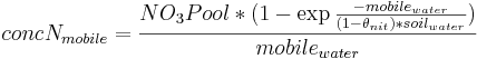
Stickstoffkonzentration des mobilen Wassers
Für die Simulation des Stofftransports mit der Wasserbewegung wird zunächst die Stickstoffkonzentration des mobilen Wassers bestimmt. Hierbei wird vereinfachend angenommen, dass ausschließlich der Stickstoff des Nitratpools mobil ist und somit in die Berechnung eingeht. Die Wassermenge bestimmt sich aus den Bodenspeichern und den den Horizont verlassenden Wasserflüssen.

mit
= Bodennitratpool [kgN/ha]
 = Bodenwassergehalt [mm]
 = Menge an Mobilem Wasser [mm]
 = Perkolationskoeffizient; Vorgabewert = 0.2 [-]
 = Oberflächenabfluss [mm]
 = Interflow [mm]
 = Perkolation in tieferen Horizont bzw. Grundwasser [mm]
 = Infiltrations Wasser, dass in einem Zeitschritt in tiefere Schichten vordringt und somit den aktuellen Horizont "bypasst" [mm]
 = Wasser, dass durch Diffusion den Horizont verlässt [mm]
 = Fraktion des Porenvolumens von dem Anionen ausgeschlossen sind (durch positiven Ladungsüberschuss der Tonminerale); Vorgabewert = 0.05 [-]
 = Stickstoffkonzentration des mobilen Wassers [kgN/ha*mm]
Das der Einfluss des Infiltrations Wassers, dass dass in einem Zeitschritt in tiefere Schichten vordringt wird mit Hilfe eines Parameters ( ) wie folgt bestimmt. Dabei repräsentiert dieser Parameter in wie weit das "Bypasswasser" mit der Bodenmatrix interagiert oder in Makroporen an den durchflossenen Schichten vorbeifliest.
![hor_{by_{infilt}}[i-1] = \sum^{n}_{i}{hor_{by_{infilt}}} * infil_{conc_{factor}} \!](/ilmswiki/uploads/math/2/9/5/29521387268f9a1f06a8919346e9fc41.png)
mit
= Infiltrations Wasser, dass in einem Zeitschritt in tiefere Schichten vordringt und somit den aktuellen Horizont "bypasst" [mm]
 = Bypassparameter [mm]
= Aktueller Horizont [-]
= Anzahl der Horizonte [-]
Stickstofftransport in den Abflusskomponenten
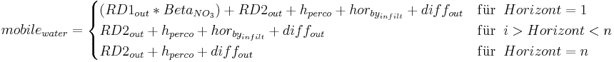
Basierend auf der Stickstoffkonzentration des mobilen Wassers werden für die einzelnen Horizonte die Stickstofffrachten für die Abflusskomponenten berechnet. Hierbei wird der Interflow in allen Horizonten und der Oberflächenabfluss nur im obersten Horizont berücksichtigt, während die Perkolation immer in den tiefer gelegenen Horizont bzw. in die Grundwasserspeicher erfolgt.


mit
= Stickstoffkonzentration des mobilen Wassers [kgN/ha*mm]
= Infiltrations Wasser, dass in einem Zeitschritt in tiefere Schichten vordringt und somit den aktuellen Horizont "bypasst" [mm]
 = Stickstoff im Oberflächenabfluss [kgN/ha]
 = Stickstoff im Interflow [kgN/ha]
 = Stickstoff im Perkolationswasser [kgN/ha]
= Oberflächenabfluss [mm]
= Interflow [mm]
= Perkolation [mm]
 = Percolationskoeffizient [-]
Der Perkolationskoeffizient stellt dabei ein Maß für die Interaktion des Oberflächenabfluss mit der Bodenmatrix des obersten Horizontes dar und Bestimmt somit den Stickstoffgehalt des Oberflächenabflusses.
Der Stoff der mit dem Diffusionswasser den Horizont verlässt wird wie folgt berechnet. Als Diffusion wird dabei die Wasserbewegung bezeichnet die aufgrund von Potentialgradienten oberhalb der Feldkapazität stattfindet. Ein negativer Wert für das Diffusionswasser bedeutet hierbei eine absteigende Wasserbewegung während ein positiver Wert eine aufsteigende Wasserbewegung repräsentiert.
![diffoutN =
\begin{cases}
w_{l_{diff}}[i] * ConcN_{mobile}[i] & \mathrm{f\ddot{u}r} \; \; w_{l_{diff}} < 0 \\
w_{l_{diff}}[i] * ConcN_{mobile}[i+1] & \mathrm{f\ddot{u}r} \; \; w_{l_{diff}} < 0
\end{cases}](/ilmswiki/uploads/math/5/2/d/52d8953e30a1b04c6d9dd799c9a047e4.png)
und
![NO_3Pool[i] = NO_3Pool[i] + diffoutN \!](/ilmswiki/uploads/math/7/b/5/7b57cb1ca33cde9ac1002c2b7af7788c.png)
und
![NO_3Pool[i+1] = NO_3Pool[i+1] - diffoutN \!](/ilmswiki/uploads/math/8/d/a/8da310efcecc92e2ec1b314ec8d885d8.png)
mit
= Stickstoffkonzentration des mobilen Wassers [kgN/ha*mm]
 = Stickstoff im Diffussionswasser [kgN/ha]
= Bodennitratpool [kgN/ha]
 = Diffussionswasser [mm]
= Bodenhorizont [kgN/ha]
Bodentemperaturmodul
Für die Stoffhaushaltsmodellierung ist die Bodentemperatur eine bedeutende Steuergröße. Insbesondere mikrobiologische Prozesse wie Nitrifikation, Denitrifikation und Umsetzung von organischem Stickstoff in der Bodenzone werden stark von der vorherrschenden Temperatur beeinflusst. Auch in dem hier erstellten Modell J2K-S spielt die Bodentemperatur bei der Berechnung der folgenden Prozesse eine Rolle (vgl. Bodenstickstoffmodul):
• Nitrifikation
• Volatilation
• Umsetzung organischer Substanz
• Abbau von Pflanzenresten
• Denitrifikation
Aufbau des Moduls
Die Bodentemperatur wird in Anlehnung an die empirischen Routinen von SWAT (Arnold et al. 1998) und EPIC (Williams et al. 1984) simuliert. Zunächst wird aus der Lufttemperatur und der Einstrahlung eine Bodenoberflächentemperatur für unbewachsenen Boden ermittelt. Diese Oberflächentemperatur wird durch Dämpfungsfaktoren, die die Wirkung von Biomasse und Schnee beschreiben, modifiziert. Die Temperatur der verschiedenen Bodenhorizonte wird zwischen der Bodenoberflächentemperatur als obere Randbedingung und der langjährigen mittleren Temperatur als untere Randbedingung ermittelt. Hierbei wird die Dämpfungswirkung des Bodens unter Berücksichtigung der Bodenfeuchte und der Lagerungsdichte bestimmt. Die Gleichungen für die einzelnen Prozesse finden sich bei Neitsch et al. (2002).
Abbildung 1: Struktur des Bodentemperaturmoduls
Abbildung 2: Ergebnisse der Bodentemperaturmodellierung für die Bodenoberfläche und in 40 cm Tiefe an einem Testhang bei Zeulenroda (Thüringen).
Die Abbildung zeigt die gemessene und modellierte Temperatur an der Bodenoberfläche (oberes Bild) sowie in 40 cm Tiefe (unteres Bild) für ein Testfeld in der nähe der Talsperre Zeulenroda. Es ist erkennbar, dass trotz gewisser Abweichungen der Temperaturverlauf gut nachvollzogen wird. Dies wird durch die hohen Bestimmtheitsmaße von rund 0.95 noch unterstrichen.
Pflanzenwachstumsmodul
Die Beschreibung zur Simulation des Pflanzenwachstums ist für eine Vielzahl von hydrologischen und Stofftransport-Prozessen wichtig, wie z.B. für die Interzeption oder die Stickstoffaufnahme durch den Pflanzenbestand. Das Pflanzenwachstum wird prinzipiell über die Simulation der Blattflächenentwicklung (LAI), der Lichtinterzeption und der Transformation in Biomasse gesteuert und erfolgt in Anlehnung an SWAT (Arnold et al. 1998). Dabei wird zunächst von einem potenziellen, d.h. unter optimalen Bedingungen vorliegenden, Pflanzenwachstum ausgegangen, welches unter Einbeziehung von Stressfaktoren modifiziert wird.
Temperaturentwicklung und Wärmesummen
Wichtigster Faktor für die Entwicklung des Pflanzenbestandes ist die Temperatur, deren Kennwerte für jede Pflanze unterschiedlich sind. Daher verfügt jede Pflanze über eine eigene Basistemperatur, die erreicht werden muss, um ein entsprechendes Wachstum auszulösen. Das Wachstum erhöht sich über die Optimumtemperatur bis es beim Überschreiten der Maximaltemperatur deutlich eingeschränkt wird.
Der pflanzenspezifische Wachstumsverlauf erfolgt über die Generierung der Wärmesummen (‚heat units = HU’). Die zugrunde liegende Hypothese hierfür beruht auf der Annahme, dass Pflanzen einen spezifischen Wärmebedarf haben, der bis zum Erreichen des Erntezustands quantifizierbar ist. Eine ‚HU’ ist als eine phänologisch wirksame Temperatureinheit definiert. Sie ergibt sich aus der täglich akkumulierten Tagesdurchschnittstemperatur, die oberhalb der pflanzenspezifischen Basistemperatur liegt. Besitzt eine Maispflanze z.B. eine Basistemperatur von 7° C und unterliegt einer Tagestemperatur von 15° C, so ergeben sich für diesen Fall 15 – 7 = 8 HU's. Auf diese Weise werden, unter Bekanntgabe der Aussaat- und Erntezeitpunkte sowie der täglichen Mittelwertstemperaturen, die individuellen Wärmesummenentwicklungen für jede Landnutzungsart simuliert. Anhand der Wärmesummenentwicklung wird der Entwicklungsverlauf des Wurzelwachstums und des Blattflächenindex gesteuert. Hierbei wird vereinfachend davon ausgegangen, dass die Pflanzen zunächst ihre Enregie in die Blattentwicklung und das Wurzelwachstum investieren. Diese Vereinfachung bedeutet auch, dass die Entwicklung von Blättern und Wurzeln unabhängig von der Wasser- und Nährstoffversorgung simuliert wird. Weiterhin wird der Reifegrad der Pflanze, der den maximalen Stickstoffgehalt in der Biomasse beeinflusst, ausschließlich über die Temperatursumme gesteuert.
Biomasseentwicklung
Die Biomasseentwicklung selbst wird zunächst als potenzielle Biomasse simuliert. Steuernde Größe für die Biomasseentwicklung ist hierbei die photosyntetisch wirksame Strahlung. So wird für jeden Tag anhand der Strahlung und der Blattfläche ein potenzieller Biomassezuwachs ermittelt (vgl. Abbildung 1).

Abbildung 1: Aufbau des Pflanzenwachstumsmoduls
Dieser tägliche Biomassezuwachs wird anhand von Stressfaktoren auf den aktuellen Biomassezuwachs reduziert. Die Stressfaktoren sind hierbei Stickstoffversorgung, Temperatur und Wasserversorgung (vgl. Abbildung 2).

Abbildung 2: Aufbau des Wachstumsstresses
Der zu einem Punkt in Raum und Zeit am stärksten wirkende Stressfaktor bestimmt, nach dem Prinzip der limitierenden Faktoren, die aktuelle Biomasseentwicklung. Dies hat wiederum eine Rückwirkung auf den Stickstoffbedarf.
Landnutzungsmanagementmodul
Die Beschreibung des Landnutzungsmanagements erfolgt in Anlehnung an die Methodik im Modell SWAT (Arnold et al. 1998). Das Landnutzungsmanagementmodul realisiert die Möglichkeit komplexe Fruchtfolgen in J2k-S darzustellen. Ausgehend von Managementoperationen wie Aussaat, Düngung und Ernte werden einzele Feldfrüchte charakterisiert. Wie in Abbildung 1 dargestellt, bezieht sich die Fruchtfolge auf eine aktuelle Pflanze, die sich wiederum aus den Pflanzenparametern und den einzelnen Managementoptionen zusammensetzt.
Bild:Pflanzenmanagementmodul1.jpg
Abbildung 1: Funktionsschema des Landnutzungsmanagementmoduls
Die grundlegenden Bausteine (Basisobjekte) zur Beschreibung des Landnutzungsmanagements sind Bodenbearbeitung (bisher noch ohne Funktion), Düngung, Pflanzeneigenschaften und die Fruchtfolge selbst. Während die Managementoptionen Bodenbearbeitung und Düngung mit einfachen Parametern wie Durchmischungseffizienz, Bearbeitungstiefe, Düngemenge, Ammonium- und Nitratanteil auskommen, ist das Pflanzenobjekt mit zahlreichen Parametern versehen. Die Fruchtfolge ist dann nur noch eine einfache Liste mit der Reihenfolge der einzelnen Feldfrüchte (vgl. Abbildung 2).
Bild:Pflanzenmanagementmodul2.jpg
Abbildung 2: Grundlegenden Bausteine (Basisobjekte)
Zur Erläuterung ist in Abbildung 3 ein Ausschnitt einer Managementparameterdatei dargestellt. In der ersten Zeile findet sich eine Bodenbearbeitungsmaßnahme. Darauf folgt die Aussaat des im Beispiel verwendeten Maises. Es finden weiterhin 3 Düngemaßnahmen mit verschiedenen Düngern statt. Weiterhin ist die Ernte mit dem geernteten Anteil der Biomasse angegeben. Der Rest verbleibt auf dem Feld und wird dem Residuen-Pool im Bodenstickstoffmodul zugeführt. Zum Abschluss findet in diesem Beispiel noch eine Bodenbearbeitung statt.
Bild:Pflanzenwaschtumsmodul4.jpg
Abbildung 3: Aufbau einer Managementparameterdatei
Mit diesem Modul ist es möglich, die wesentlichen Tätigkeiten des pflanzenbaulichen Management flexibel abzubilden und Managementalternativen darzustellen.
Grundwasserstickstoffmodul
Die Beschreibung der Dynamik des Stickstoffes im Grundwasser wird in Anlehnung an die in J2k verwendete Grundwasserdynamik durchgeführt. Hierbei wird die Stofffracht entsprechend der Verteilung des Wassers auf die beiden Grundwasserspeicher RG1 und RG2 aufgeteilt. Es werden für beide Grundwasserspeicher getrennt die Wasser- und Stoffgehalte ermittelt. Die Abgabe erfolgt analog zum Wasser und den ermittelten Gehalten. Es ist möglich eine Anfangsstickstoffkonzentration vorzugeben.
Auserdem wurde noch ein Dämpfungsfaktor implementiert, der die Änderung der Stickstoffgehalte im Speicher verzögert. Dieser, zur Kalibration verwendbare Faktor, ist für beide Grundwasserspeicher getrennt einstellbar. Er repräsentiert Durchmischungs- und Diffusionseffekte im Grundwasserleiter.
Zurück zu Modelle