Water and Nutrient Balance Model J2000-S
(→Transfer zwischen den organischen Pools) |
(→Soil Temperature Module) |
||
| (40 intermediate revisions by 2 users not shown) | |||
| Line 1: | Line 1: | ||
| − | + | [[de:Wasser-_und_Stofftransportmodell_J2000-S]] | |
| + | The water and nutrient balance model J2000-S offers a simulation of the water and nitrogen balance of meso scale catchment areas. The model is an extension to the [[Hydrological_Model_J2000|J2000]] model with which it shares most of the components for the description of the hydrologic cycle. The additional components, soil temperature, soil nitrogen balance, land use management, plant growth as well as ground water nitrogen balance, are described for the specification of the nitrogen balance. Further modules are adapted for the demands of the nitrogen balance. | ||
---- | ---- | ||
| − | == | + | ==Soil Nitrogen Module== |
| − | + | The description of the soil nitrogen balance is carried out similarly to the SWAT model (Arnold et al. 1998). Within the individual soil horizons the five nitrogen pools for nitrate, ammonium, stable organic substances, active organic substance and fresh plant remains as biomass are distinguished. The fluxes and transformations between the pools and outside the soil, like nitrification, denitrification, mineralization, volatilation, plant uptake and eluviation, are calculated via the empirical relations against the soil humidity and soil temperature. The nitrogen flux is passed as well as the water transport via a routing method between the subareas to the receiving stream (see figure 1). | |
| − | + | The nitrogen input caused by fertilization and Bestandesabfall as well as the removal through the plants is provided by the plant growth module and the land use management module. The mineral inputs are allocated to the ammonium pool or directly to the nitrate pool. The organic nitrogen is either allocated to the Bestandesabfall pool or the active organic pool. The latter is poised with the stable organic pool. The nitrate pool is the central allocation section for the discharge as eluviation, plant uptake and denitrification. The processes described in the module take place in free parameterizable soil horizons. Here, the delivery of organic substances and fertilizer as well as the removal of nitrogen with the surface runoff are limited to the top horizon. | |
| − | + | ||
| Line 16: | Line 16: | ||
Figure 1: Structure of the soil nitrogen module | Figure 1: Structure of the soil nitrogen module | ||
| − | The here applied nitrogen module contains some simplifications. Thus, no | + | The here applied nitrogen module contains some simplifications. Thus, no plant uptake from the ammonium pool is offered. Furthermore, the decomposition of organic substances is directly simulated to nitrate without any detour via ammonium. The N immobilization from mineral to organic nitrogen in the soil zone is neglected completely. The water transport of nitrogen is shown very generalized. Thus, a complete mixing of nitrogen in the individual storages takes place instead of advection and dispersion. The individual processes are described in the model as follows: |
| − | === | + | ===Plant Uptake=== |
| − | At first, the plant’s demands (potential | + | At first, the plant’s demands (potential plant uptake) which shall be met by the soil nitrogen storage on the day t0 are generated: |
<math> potNup= BioNopt - BioN \! </math> [1] | <math> potNup= BioNopt - BioN \! </math> [1] | ||
| Line 27: | Line 27: | ||
with: | with: | ||
| − | '' <math>potNup\!</math> = potential | + | '' <math>potNup\!</math> = potential plant uptake [kgN/ha]'' |
'' <math>BioNopt\!</math> = optimal biomass [kgN/ha]'' | '' <math>BioNopt\!</math> = optimal biomass [kgN/ha]'' | ||
| Line 33: | Line 33: | ||
'' <math>BioN\!</math> = actual biomass [kgN/ha]'' | '' <math>BioN\!</math> = actual biomass [kgN/ha]'' | ||
| − | Afterwards, the proportions of the soil horizons which lie within the effective root zone are generated. At this, the horizons which lie | + | Afterwards, the proportions of the soil horizons which lie within the effective root zone are generated. At this, the horizons which lie entirely within the root zone are taken into account completely (partroot = 1). However, the horizon which lies only partly in the root zone is only considered partly: |
<math> partroot[i] = \frac {rootdepth - layerdepth[i - 1]}{layerdepth[i] - layerdepth[i - 1]} \! </math> [2] | <math> partroot[i] = \frac {rootdepth - layerdepth[i - 1]}{layerdepth[i] - layerdepth[i - 1]} \! </math> [2] | ||
| Line 51: | Line 51: | ||
with: | with: | ||
| − | '' <math>i\!</math> = | + | '' <math>i\!</math> = horizon [-] '' |
'' <math>partroot\!</math> = proportion of the horizon at the root zone [-]'' | '' <math>partroot\!</math> = proportion of the horizon at the root zone [-]'' | ||
| Line 57: | Line 57: | ||
'' <math>layerdepth\!</math> = lower threshold of the soil horizon [-]'' | '' <math>layerdepth\!</math> = lower threshold of the soil horizon [-]'' | ||
| − | '' <math>potNup\!</math> = potential | + | '' <math>potNup\!</math> = potential plant uptake [kgN/ha]'' |
| − | '' <math>potNup_z\!</math> = potential | + | '' <math>potNup_z\!</math> = potential plant uptake in the individual horizons [kgN/ha]'' |
| − | '' <math>uptake\!</math> = potential | + | '' <math>uptake\!</math> = potential plant uptake which has been taken from upper horizons already [kgN/ha]'' |
| − | '' <math>\beta_{Ndist}\!</math> = distribution parameter of the | + | '' <math>\beta_{Ndist}\!</math> = distribution parameter of the plant uptake; default value = 1.0; possible values 1 - 15 [-]'' |
| − | For the calculation of the potential | + | For the calculation of the potential plant uptake which is met by upper horizons already, the following connection is applied: |
<math> uptake = uptake + potNup_z[i] \! </math> [4] | <math> uptake = uptake + potNup_z[i] \! </math> [4] | ||
| − | '' <math>potNup_z\!</math> = potential | + | '' <math>potNup_z\!</math> = potential plant uptake in the individual horizons [kgN/ha]'' |
| − | '' <math>uptake\!</math> = potential | + | '' <math>uptake\!</math> = potential plant uptake which has been taken from upper horizons already [kgN/ha]'' |
| Line 87: | Line 87: | ||
'' <math>NO_3Pool\!</math> = soil nitrogen pool [kgN/ha]'' | '' <math>NO_3Pool\!</math> = soil nitrogen pool [kgN/ha]'' | ||
| − | '' <math>potNup_z\!</math> = potential | + | '' <math>potNup_z\!</math> = potential plant uptake in the individual horizons [kgN/ha]'' |
If this demand is greater than 0, it can be met by the existing nitrogen storage with: | If this demand is greater than 0, it can be met by the existing nitrogen storage with: | ||
| Line 119: | Line 119: | ||
'' <math>NO_3Pool2\!</math> = soil nitrate pool after the time step [kgN/ha]'' | '' <math>NO_3Pool2\!</math> = soil nitrate pool after the time step [kgN/ha]'' | ||
| − | '' <math>potNupz\!</math> = potential | + | '' <math>potNupz\!</math> = potential plant uptake in the individual horizons [kgN/ha]'' |
'' <math>partroot\!</math> = proportion of the horizon of the root zone [-]'' | '' <math>partroot\!</math> = proportion of the horizon of the root zone [-]'' | ||
| − | + | Aterwards, the actual plant uptake can be calculated on the basis of the potential plant uptake and the demand that has been summed up via the horizons: | |
<math> N_{uptake} = potNup + \sum^{n}_{i=1}{demand[i]} \! </math> [10] | <math> N_{uptake} = potNup + \sum^{n}_{i=1}{demand[i]} \! </math> [10] | ||
| Line 132: | Line 132: | ||
'' <math>i\!</math> = horizon [-] '' | '' <math>i\!</math> = horizon [-] '' | ||
| − | '' <math>n\!</math> = | + | '' <math>n\!</math> = number of horizons in the root zone [-] '' |
'' <math>demand\!</math> = demand which can be met by the soil nitrogen pool [kgN/ha]'' | '' <math>demand\!</math> = demand which can be met by the soil nitrogen pool [kgN/ha]'' | ||
| − | '' <math>potNup\!</math> = potential | + | '' <math>potNup\!</math> = potential plant uptake [kgN/ha]'' |
| − | '' <math>N_{uptake}\!</math> = actual | + | '' <math>N_{uptake}\!</math> = actual plant uptake [kgN/ha]'' |
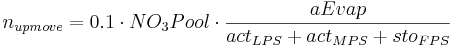
===Nitrate Rising by Evaporation=== | ===Nitrate Rising by Evaporation=== | ||
| Line 172: | Line 172: | ||
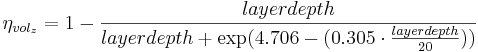
'' <math>\eta_{temp}\!</math> = soil temperature coefficient [-]'' | '' <math>\eta_{temp}\!</math> = soil temperature coefficient [-]'' | ||
| − | '' <math>temp_{Layer}\!</math> = | + | '' <math>temp_{Layer}\!</math> = temperature of the soil layer [°C]'' |
| Line 187: | Line 187: | ||
with | with | ||
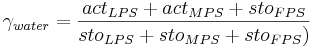
| − | '' <math> \eta_{water}\! </math> = soil humidity coefficient[-]'' | + | '' <math> \eta_{water}\! </math> = soil humidity coefficient [-]'' |
'' <math>sto_{LPS}\!</math> = maximum large pore storage of the horizon [l]'' | '' <math>sto_{LPS}\!</math> = maximum large pore storage of the horizon [l]'' | ||
| Line 208: | Line 208: | ||
'' <math>layerdepth\!</math> = layer depth of the horizon [cm]'' | '' <math>layerdepth\!</math> = layer depth of the horizon [cm]'' | ||
| − | The | + | The Gesamtumsatz of the ammonium pool can be calculated as follows: |
<math> N_{nit + vol} = NH_4Pool * (1 - \exp(-(\eta_{water} \cdot \eta_{temp})-(\eta_{vol_z} \cdot \eta_{temp})))\!</math> | <math> N_{nit + vol} = NH_4Pool * (1 - \exp(-(\eta_{water} \cdot \eta_{temp})-(\eta_{vol_z} \cdot \eta_{temp})))\!</math> | ||
| Line 238: | Line 238: | ||
'' <math>frac_{vol}\!</math> = fraction ammonium volatilation [-]'' | '' <math>frac_{vol}\!</math> = fraction ammonium volatilation [-]'' | ||
| − | '' <math>nitri_{trans}\!</math> = amount of | + | '' <math>nitri_{trans}\!</math> = amount of nitrification [kgN/ha]'' |
| − | '' <math>volati_{trans}\!</math> = amount of | + | '' <math>volati_{trans}\!</math> = amount of ammonium volatilation [kgN/ha]'' |
| − | ====Pre-calculation for the Influence of | + | ====Pre-calculation for the Influence of Environmental Conditions==== |
| − | In order to show the influence of the soil temperature and | + | In order to show the influence of the soil temperature and soil humidity in the different transformation processes, the following coefficients need to be calculated beforehand: U |
<math> \gamma_{temp} = 0.9 \cdot \frac {temp_{Layer}} {temp_{Layer} \cdot \exp(9.93 - 0.312 \cdot temp_{Layer}} + 0.1 \! </math> [1] | <math> \gamma_{temp} = 0.9 \cdot \frac {temp_{Layer}} {temp_{Layer} \cdot \exp(9.93 - 0.312 \cdot temp_{Layer}} + 0.1 \! </math> [1] | ||
| Line 272: | Line 272: | ||
'' <math>act_{MPS}\!</math> = actual middle pore storage of the horizon [l]'' | '' <math>act_{MPS}\!</math> = actual middle pore storage of the horizon [l]'' | ||
| + | |||
====Transfer between the Organic Pools==== | ====Transfer between the Organic Pools==== | ||
| Line 281: | Line 282: | ||
with | with | ||
| − | '' <math>N_{Hum_{trans}}\!</math> = transfer rate between the active and | + | '' <math>N_{Hum_{trans}}\!</math> = transfer rate between the active and stable organic pool [kgN/ha]'' |
| − | '' <math>\beta_{trans}\!</math> = transfer constant between the active and | + | '' <math>\beta_{trans}\!</math> = transfer constant between the active and stable organic pool; default value= 0.00001 [-]'' |
'' <math>N_{activ_{pool}}\!</math> = active organic pool [kgN/ha]'' | '' <math>N_{activ_{pool}}\!</math> = active organic pool [kgN/ha]'' | ||
| Line 293: | Line 294: | ||
The transfer rate is here subtracted from the active pool whereas it is added to the stable pool. | The transfer rate is here subtracted from the active pool whereas it is added to the stable pool. | ||
| − | ==== | + | ====Mineralization of the Active Pool==== |
| − | + | The active pool is mineralized to nitrate directly without taking the nitrification into account. The rate is calculated as follows: | |
<math>N_{actmin} = \beta_{min} \cdot \sqrt{\gamma_{temp} \cdot \gamma_{water}} \cdot N_{activ_{pool}}\!</math> | <math>N_{actmin} = \beta_{min} \cdot \sqrt{\gamma_{temp} \cdot \gamma_{water}} \cdot N_{activ_{pool}}\!</math> | ||
| − | + | with | |
| − | '' <math>N_{actmin}\!</math> = | + | '' <math>N_{actmin}\!</math> = transfer rate between the active organic and the nitrate pool [kgN/ha]'' |
| − | '' <math>\beta_{min}\!</math> = | + | '' <math>\beta_{min}\!</math> = transfer constant between the active organic and the nitrate pool; default value = 0.002 [-]'' |
| − | '' <math>N_{activ_{pool}}\!</math> = | + | '' <math>N_{activ_{pool}}\!</math> = active organic pool [kgN/ha]'' |
| − | '' <math>\gamma_{water}\!</math> = | + | '' <math>\gamma_{water}\!</math> = soil humidity coefficient [-]'' |
| − | '' <math>\gamma_{temp}\!</math> = | + | '' <math>\gamma_{temp}\!</math> = soil temperature coefficient [-]'' |
| − | + | The transfer rate is subtracted from the active pool whereas it is added to the nitrate pool. | |
| − | ==== | + | ====Dynamics of the Residue Pools==== |
| − | + | The dynamics of the decomposition of fresh organic substances (residue) from plant remains and organic fertilizer is carried out only in the top horizon. The residue are divided in two pools: the first one represents the biomass as a whole, the second represents the residue's amount of nitrogen. The supply to the residue pools is carried out via plant remains after the harvest and via the organic fertilization with the help of the following equation: | |
<math>Residue_{pool} = Residue_{pool} + inp_{biomass} + (fertorgN_{fresh} \cdot 10)\! </math> | <math>Residue_{pool} = Residue_{pool} + inp_{biomass} + (fertorgN_{fresh} \cdot 10)\! </math> | ||
| Line 322: | Line 323: | ||
<math>N_{residue_{pool}} = N_{residue_{pool}} + inpN_{biomass} + fertorgN_{fresh}\!</math> | <math>N_{residue_{pool}} = N_{residue_{pool}} + inpN_{biomass} + fertorgN_{fresh}\!</math> | ||
| − | + | with | |
| − | '' <math>Residue_{pool}\!</math> = | + | '' <math>Residue_{pool}\!</math> = residue pool [kg/ha]'' |
| − | '' <math>inp_{biomass}\!</math> = | + | '' <math>inp_{biomass}\!</math> = inputted biomass [kg/ha]'' |
| − | '' <math>fertorgN_{fresh}\!</math> = | + | '' <math>fertorgN_{fresh}\!</math> = inputted nitrogen via organic fertilization [kgN/ha]'' |
| − | '' <math>N_{residue_{pool}}\!</math> = | + | '' <math>N_{residue_{pool}}\!</math> = residue pool's amount of nitrogen [kgN/ha]'' |
| − | + | The decomposition of the residue pool is carried out against the carbon-nitrogen relation (C/N-relation). The calculation of the C/N-relation is carried out according to the following equation. | |
<math>\epsilon_{C/N} = \frac{Residue_{pool} \cdot 0.58} {N_{residue_{pool}} + NO_3Pool}</math> | <math>\epsilon_{C/N} = \frac{Residue_{pool} \cdot 0.58} {N_{residue_{pool}} + NO_3Pool}</math> | ||
| Line 345: | Line 346: | ||
| − | + | with | |
| − | '' <math>\epsilon_{C/N}\!</math> = C/N- | + | '' <math>\epsilon_{C/N}\!</math> = C/N-relation [-]'' |
| − | '' <math>\gamma_{ntr}\!</math> = | + | '' <math>\gamma_{ntr}\!</math> = residue decomposition factor [-]'' |
| − | '' <math>Residue_{pool}\!</math> = | + | '' <math>Residue_{pool}\!</math> = residue pool [kg/ha]'' |
| − | '' <math>NO_3Pool\!</math> = | + | '' <math>NO_3Pool\!</math> = nitrate pool [kgN/ha]'' |
| − | '' <math>N_{residue_{pool}}\!</math> = | + | '' <math>N_{residue_{pool}}\!</math> = residue pool's amount of nitrogen [kgN/ha]'' |
| − | + | The decomposition constant of the residue pool is calculated with <math>\gamma_{ntr}</math>, <math>\gamma_{water}</math>, <math>\gamma_{temp}</math>: | |
'' <math>\delta_{ntr} = \beta_{rsd} \cdot \gamma_{ntr} \cdot \sqrt{\gamma_{water} \cdot \gamma_{temp}}\!</math> | '' <math>\delta_{ntr} = \beta_{rsd} \cdot \gamma_{ntr} \cdot \sqrt{\gamma_{water} \cdot \gamma_{temp}}\!</math> | ||
| − | + | with | |
| − | '' <math>\delta_{ntr}\!</math> = | + | '' <math>\delta_{ntr}\!</math> = constant of the residue decomposition’s rate [-]'' |
| − | '' <math>\gamma_{ntr}\!</math> = | + | '' <math>\gamma_{ntr}\!</math> = residue decomposition factor [-]'' |
| − | '' <math>\beta_{rsd}\!</math> = | + | '' <math>\beta_{rsd}\!</math> = residue decomposition coefficient; default value = 0.05 [-]'' |
| − | '' <math>\gamma_{water}\!</math> = | + | '' <math>\gamma_{water}\!</math> = soil humidity coefficient [-]'' |
| − | '' <math>\gamma_{temp}\!</math> = | + | '' <math>\gamma_{temp}\!</math> = soil temperature coefficient [-]'' |
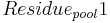
| − | + | The decomposition of the residue pool is carried out with the constant of the residue decomposition’s rate. At this, the nitrogen part is allocated to the active organic pool, in terms of humification, and the nitrate pool, in terms of mineralization, in a ratio of 20:80. | |
<math>Residue_{pool}2 = Residue_{pool}1 - (\delta_{ntr} \cdot Residue_{pool}1)\!</math> | <math>Residue_{pool}2 = Residue_{pool}1 - (\delta_{ntr} \cdot Residue_{pool}1)\!</math> | ||
| Line 385: | Line 386: | ||
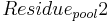
<math>N_{residue_{pool}}2 = N_{residue_{pool}}1 - (\delta_{ntr} \cdot N_{residue_{pool}}1)\!</math> | <math>N_{residue_{pool}}2 = N_{residue_{pool}}1 - (\delta_{ntr} \cdot N_{residue_{pool}}1)\!</math> | ||
| − | + | with | |
| − | '' <math>\delta_{ntr}\!</math> = | + | '' <math>\delta_{ntr}\!</math> = constant of the residue decomposition’s rate [-]'' |
| − | '' <math>Residue_{pool}1\!</math> = | + | '' <math>Residue_{pool}1\!</math> = residue pool before the time step [kgN/ha]'' |
| − | '' <math>Residue_{pool}2\!</math> = | + | '' <math>Residue_{pool}2\!</math> = residue pool after the time step [kgN/ha]'' |
| − | '' <math>N_{active_{pool}}1\!</math> = | + | '' <math>N_{active_{pool}}1\!</math> = active organic pool before the time step [kgN/ha]'' |
| − | '' <math>N_{active_{pool}}2\!</math> = | + | '' <math>N_{active_{pool}}2\!</math> = active organic pool after the time step [kgN/ha]'' |
| − | '' <math>NO_3Pool1\!</math> = | + | '' <math>NO_3Pool1\!</math> = soil nitrate pool before the time step [kgN/ha]'' |
| − | '' <math>NO_3Pool2\!</math> = | + | '' <math>NO_3Pool2\!</math> = soil nitrate pool after the time step [kgN/ha]'' |
| − | '' <math>N_{residue_{pool}}1\!</math> = | + | '' <math>N_{residue_{pool}}1\!</math> = residue pool's amount of nitrogen before the time step [kgN/ha]'' |
| − | '' <math>N_{residue_{pool}}2\!</math> = | + | '' <math>N_{residue_{pool}}2\!</math> = residue pool's amount of nitrogen after the time step [kgN/ha]'' |
| − | ==== | + | ====Denitrification==== |
| − | + | Denitrification occurs when the soil is nearly water-saturated. The rate depends on the amount of organic carbon in the soil as well as on the soil temperature. In comparison to SWAT (0,95), the degree of water saturation is lower (0.91) when denitrification occurs. This is because SWAT - in contrast to J2000 - does not consider the soil's air capacity. Thus, the underlying pore volume for the calculation of water saturation is higher in J2000. Furthermore, it is ensured that the rate is at the most 1 kgN/ha*d since higher rates are not expected in open land. | |
| Line 418: | Line 419: | ||
</math> | </math> | ||
| − | + | with | |
| − | '' <math>NO_3Pool\!</math> = | + | '' <math>NO_3Pool\!</math> = soil nitrate pool [kgN/ha]'' |
| − | '' <math>denit_{trans}\!</math> = | + | '' <math>denit_{trans}\!</math> = denitrification rate [kgN/ha]'' |
| − | '' <math>\gamma_{water}\!</math> = | + | '' <math>\gamma_{water}\!</math> = soil humidity coefficient [-]'' |
| − | '' <math>\gamma_{temp}\!</math> = | + | '' <math>\gamma_{temp}\!</math> = soil temperature coefficient [-]'' |
| − | '' <math>\beta_{denit}\!</math> = | + | '' <math>\beta_{denit}\!</math> = denitrification coefficient; default value = 0.91 [-]'' |
| − | |||
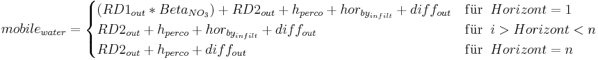
| − | === | + | ===Mass Transport with Water Movement in the Soil=== |
| + | ====Nitrogen Concentration of Mobile Water==== | ||
| − | + | ||
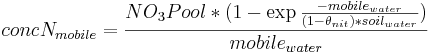
| + | For the simulation of the mass transport caused by water movement, the nitrogen concentration of the mobile water is defined. Here, it is simplified assumed that only the nitrogen of the nitrate pool is mobile and therefore is taken into account for the calculation. The amount of water is determined on the basis of the soil storages and the water streams that leave the horizon. | ||
| Line 451: | Line 453: | ||
<math>concN_{mobile} = \frac {NO_3Pool * (1 - \exp \frac{- mobile_{water}} {(1 - \theta_{nit}) * soil_{water}})} {mobile_{water}}</math> | <math>concN_{mobile} = \frac {NO_3Pool * (1 - \exp \frac{- mobile_{water}} {(1 - \theta_{nit}) * soil_{water}})} {mobile_{water}}</math> | ||
| − | + | with | |
| − | '' <math>NO_3Pool\!</math> = | + | '' <math>NO_3Pool\!</math> = soil nitrate pool [kgN/ha]'' |
| − | '' <math>soil_{water}\!</math> = | + | '' <math>soil_{water}\!</math> = soil water [mm]'' |
| − | '' <math>mobile_{water}\!</math> = | + | '' <math>mobile_{water}\!</math> = amount of mobile water [mm]'' |
| − | '' <math>\Beta_{NO_{3}}\!</math> = | + | '' <math>\Beta_{NO_{3}}\!</math> = percolation coefficient; default value = 0.2 [-] '' |
| − | '' <math>RD1_{out}\!</math> = | + | '' <math>RD1_{out}\!</math> = surface runoff [mm]'' |
| − | '' <math>RD2_{out}\!</math> = | + | '' <math>RD2_{out}\!</math> = interflow [mm]'' |
| − | '' <math>h_{perco}\!</math> = | + | '' <math>h_{perco}\!</math> = percolation in deeper horizons or ground water [mm]'' |
| − | '' <math>hor_{by_{infilt}}\!</math> = | + | '' <math>hor_{by_{infilt}}\!</math> = infiltration water that goes into deeper layers in a time step and therefore passes by the actual horizon [mm]'' |
| − | '' <math>diff_{out}\!</math> = | + | '' <math>diff_{out}\!</math> = water that leaves the horizon via diffusion [mm]'' |
| − | '' <math>\theta_{nit}\!</math> = | + | '' <math>\theta_{nit}\!</math> = fraction of the pore volume from which anions are excluded (due to positive charge preponderance of the clay mineral); default value = 0.05 [-]'' |
| − | '' <math> concN_{mobile}\!</math> = | + | '' <math> concN_{mobile}\!</math> = nitrogen concentration of the mobile water [kgN/ha*mm]'' |
| − | + | The influence of the water that expands into deeper horizons in a time step is determined with a parameter (<math>infil_{conc_{factor}}</math>). At this, the parameter represents to what extend the bypass water interacts with the soil matrix or bypasses the layers that are flown through in macro pores. | |
<math>hor_{by_{infilt}}[i-1] = \sum^{n}_{i}{hor_{by_{infilt}}} * infil_{conc_{factor}} \!</math> | <math>hor_{by_{infilt}}[i-1] = \sum^{n}_{i}{hor_{by_{infilt}}} * infil_{conc_{factor}} \!</math> | ||
| − | + | with | |
| − | '' <math>hor_{by_{infilt}}\!</math> = | + | '' <math>hor_{by_{infilt}}\!</math> = infiltration water that goes into deeper layers in a time step and therefore passes by the actual horizon [mm]'' |
| − | '' <math>infil_{conc_{factor}}\!</math> = | + | '' <math>infil_{conc_{factor}}\!</math> = bypass parameter [mm]'' |
| − | '' <math>i\!</math> = | + | '' <math>i\!</math> = actual horizon [-]'' |
| − | '' <math>n\!</math> = | + | '' <math>n\!</math> = number of horizons [-]'' |
| − | ==== | + | ====Nitrogen Transport in the Runoff Components==== |
| − | + | For the individual horizons the nitrogen loads for the runoff components are calculated on the basis of the mobile water's nitrogen concentration. At this, the interflow is considered in all horizons whereas the surface runoff is only considered in the top horizon. However, the percolation occurs in the deeper horizons or in the ground-water reservoir. | |
| + | |||
<math>N_{surface} = Beta_{NO_3} \cdot RD1_{out} \cdot concN_{mobile}\!</math> | <math>N_{surface} = Beta_{NO_3} \cdot RD1_{out} \cdot concN_{mobile}\!</math> | ||
| Line 500: | Line 503: | ||
| − | + | with | |
| − | '' <math> concN_{mobile}\!</math> = | + | '' <math> concN_{mobile}\!</math> = nitrogen concentration of the mobile water [kgN/ha*mm]'' |
| − | '' <math>hor_{by_{infilt}}\!</math> = | + | '' <math>hor_{by_{infilt}}\!</math> = infiltration water that goes in deeper layers and thus bypasses the actual horizon in a time step [mm]'' |
| − | '' <math>N_{surface}\!</math> = | + | '' <math>N_{surface}\!</math> = nitrogen in the surface runoff [kgN/ha]'' |
| − | '' <math>N_{interflow}\!</math> = | + | '' <math>N_{interflow}\!</math> = nitrogen in the interflow [kgN/ha]'' |
| − | '' <math>N_{perco}\!</math> = | + | '' <math>N_{perco}\!</math> = nitrogen in the percolation water [kgN/ha]'' |
| − | '' <math>RD1_{out}\!</math> = | + | '' <math>RD1_{out}\!</math> = surface runoff [mm]'' |
| − | '' <math>RD2_{out}\!</math> = | + | '' <math>RD2_{out}\!</math> = interflow [mm]'' |
| − | '' <math>h_{perco}\!</math> = | + | '' <math>h_{perco}\!</math> = percolation [mm]'' |
| − | '' <math>Beta_{NO_3}\!</math> = | + | '' <math>Beta_{NO_3}\!</math> = percolation coefficient [-]'' |
| − | + | The percolation coefficient represents a measurement for the interaction of the surface runoff and the soil matrix of the top horizon and therefore determines the surface runoff's amount of nitrogen. | |
| − | + | The material that leaves the horizon with the diffusion water can be calculated as follows: the water movement that occurs above the field capacity due to potential gradients is called diffusion. Here, a negative value for the diffusion water means a downward water movement whereas a positive value represents an upward water movement. | |
| Line 533: | Line 536: | ||
</math> | </math> | ||
| − | + | and | |
<math>NO_3Pool[i] = NO_3Pool[i] + diffoutN \!</math> | <math>NO_3Pool[i] = NO_3Pool[i] + diffoutN \!</math> | ||
| − | + | and | |
<math>NO_3Pool[i+1] = NO_3Pool[i+1] - diffoutN \!</math> | <math>NO_3Pool[i+1] = NO_3Pool[i+1] - diffoutN \!</math> | ||
| − | + | with | |
| − | '' <math> concN_{mobile}\!</math> = | + | '' <math> concN_{mobile}\!</math> = nitrogen concentration of the mobile water [kgN/ha*mm]'' |
| − | '' <math>diffoutN \!</math> = | + | '' <math>diffoutN \!</math> = nitrogen in the diffusion water [kgN/ha]'' |
| − | '' <math>NO_3Pool\!</math> = | + | '' <math>NO_3Pool\!</math> = soil nitrate pool [kgN/ha]'' |
| − | '' <math>w_{l_{diff}}\!</math> = | + | '' <math>w_{l_{diff}}\!</math> = diffusion water [mm]'' |
| − | '' <math>i\!</math> = | + | '' <math>i\!</math> = soil horizon [kgN/ha]'' |
| Line 560: | Line 563: | ||
---- | ---- | ||
| − | == | + | ==Soil Temperature Module== |
| − | + | ||
| − | |||
| − | |||
| − | + | The soil temperature is an important measurement for the matter regime modeling. Especially microbiological processes such as nitrification, denitrification and the transformation of organic nitrogen in the soil zone is strongly influenced by the prevailing temperature. | |
| + | In the here developed model J2K-S the soil temperature also plays an important role for the calculation of the following processes (see [[Soil_Nitrogen_Module_empty|Soil Nitrogen Module]]): | ||
| − | • | + | • nitrification |
| − | • | + | • volatilation |
| − | • | + | • transformation of organic substance |
| − | • | + | • decomposition of plant remains |
| + | • denitrification | ||
| − | '' | + | ''Structure of the Module'' |
| − | + | The soil temperature is simulated according to the empirical routines of SWAT (Arnold et al. 1998) and EPIC (Williams et al. 1984). At first, a surface soil temperature is generated for bare ground on the basis of the air temperature and insolation. This surface temperature is modified by attenuation factors that describe the effect of biomass and snow. The temperature of the different soil horizons is generated as upper boundary condition between the surface soil temperature and the long lasting mean temperature as lower boundary condition. At this, the attenuation effect of the soil is defined in consideration of the soil humidity and the bulk density. The equations of the individual processes can be found in Neitsch et al. (2002). | |
| − | + | ||
[[Bild:Bodentemperaturmodul.jpg]] | [[Bild:Bodentemperaturmodul.jpg]] | ||
| − | + | Figure 1: Structure of the soil temperature model | |
[[Bild:Bodentemperaturtest.jpg]] | [[Bild:Bodentemperaturtest.jpg]] | ||
| − | + | Figure 2: Results of the soil temperature modeling for the surface area and at 40 cm depth at an investigated slope near Zeulenroda (Thuringia). | |
| − | + | This figure shows the measured and modeled temperature at the surface (upper figure) as well as at 40 cm depth (lower figure) for an investigated area near the dam Zeulenroda. It can be seen that the temperature curve can be followed quite well in spite of certain deviations. This is emphasized by the high coefficient of determination of about 0.95. | |
---- | ---- | ||
| − | |||
| − | + | ==Plant Growth Module== | |
| + | The description for the simulation of plant growth is important for numerous hydrological mass transport processes, e.g. for the interception or the nitrogen uptake by the canopy. Plant growth is usually controlled via the simulation of the leaf area development (LAI) as well as the light interception and the transformation into biomass and is carried out according to SWAT (Arnold et al. 1998). At this, it is assumed that a potential plant growth, i.e. under optimum conditions, exists which is then modified in consideration of stress factors. | ||
| − | |||
| + | ''Temperature Development and Heat Units'' | ||
| − | |||
| − | |||
| + | The most important factor that determines the canopy’s development is the temperature whose parameters are different for each plant. Therefore, each plant possesses a basis temperature that needs to be reached in order to activate a certain growth. The growth increases until the optimum temperature is reached and decreases noticeably when the maximum temperature is exceeded. The plant-specific growth development is carried out via the generating of heat units (=HU). The underlying hypothesis for this is the assumption that plants have a specific heat demand that is quantifiable until the necessary maturity state for the harvest is reached. An ‘HU’ is defined as a phenological effective temperature unit. An HU results from the daily accumulated daily average temperature that lies above the plant-specific basis temperature. Assumed that a maize plant has a basis temperature of 7° C and is exposed to a daily temperature of 15° C, its HU would be calculated as follows: 15 – 7 = 8 HUs. In this way, the individual heat unit developments are simulated for each land use type in consideration of the time of the sowing and harvest as well as the daily average temperature. The development of the root growth and the leaf area index is controlled via the heat unit development. At this, it is assumed that the plants invest their energy into the leaf development and the root growth. This simplified view also means that the development of leafs and roots is independent on water and nutrient supply. Furthermore, the plant’s degree of maturity which influences the amount of nitrogen in the biomass is exclusively controlled via the temperature sum. | ||
| − | |||
| + | ''Biomass Development '' | ||
| − | + | ||
| + | The biomass development is simulated as potential biomass at first. At this, the photosyntetic radiation is the controlling unit for the biomass development. Thus, a potential biomass increase is generated for each day with the help of the radiation and leaf area (see figure 1). | ||
[[image:Pflanzenwastumsmodul1.jpg]] | [[image:Pflanzenwastumsmodul1.jpg]] | ||
| − | + | Figure 1: Structure of the plant growth module | |
| − | + | This daily biomass increase is reduced to the actual biomass increase with the help of stress factors, which are nitrogen supply, temperature and water supply (see figure 2). | |
[[image:Pflanzenwastumsmodul2.jpg]] | [[image:Pflanzenwastumsmodul2.jpg]] | ||
| − | + | Figure 2: Structure of the growth’s stress | |
| − | + | The stress factor that has the strongest effects at a point in space and time determines the actual biomass according to the principle of limiting factors. This, in turn, influences the nitrogen demand. | |
---- | ---- | ||
| − | |||
| − | + | ==Land Use Management Module== | |
| + | |||
| + | The description of the land use management is carried out according to the methodology in the SWAT model (Arnold et al. 1998). The land use management module offers to represent complex crop rotations in J2k-S. The individual field crops are characterized on the basis of management operations like sowing, fertilizing and harvesting. As can be seen in figure 1, the crop rotation relates to an actual plant that in turn is build up of the plant parameters and the individual management options. | ||
[[Bild:Pflanzenmanagementmodul1.jpg]] | [[Bild:Pflanzenmanagementmodul1.jpg]] | ||
| − | + | Figure 1: Flow chart of the land use management module | |
| − | + | The basic basis objects for the description of the land use management are cultivation (no function yet), fertilization, plant characteristics and the crop rotation. Land management and fertilization as management options have only simple parameters like mixing efficiency, machining depth, amount of fertilizer, ammonium and nitrate. However, the plant object possesses numerous parameters. Thus, the crop rotation is a simple list with the order of the individual crops (see figure 2). | |
| Line 646: | Line 648: | ||
[[Bild:Pflanzenmanagementmodul2.jpg]] | [[Bild:Pflanzenmanagementmodul2.jpg]] | ||
| − | + | Figure 2: Essential components (basic objects) | |
| − | + | As an explanation in figure 3 a detail of a management parameter file is shown. In the first line a cultivation type can be found. Thereupon, the sowing of the maize that was used in the example follows. Furthermore, three fertilizations with three different fertilizers are carried out. The harvest with the amount of biomass is given. The rest remains on the field and is allocated to the residue pool in the nitrogen module. Finally, cultivation is carried out in this example. | |
| Line 656: | Line 658: | ||
| − | + | Figure 3: Structure of a management parameter file | |
| − | + | With the help of this tool, the essential activities of the horticultural management as well as alternatives can be represented flexibly. | |
---- | ---- | ||
| − | == | + | ==Ground Water Nitrogen Module== |
| + | |||
| + | The description of the nitrogen’s dynamics that occurs in the ground water is carried out according to the ground water dynamics used in J2k. At this, the nitrogen load is – corresponding to the water – allocated to the two ground-water reservoirs RG1 and RG2. The water and matter proportions are generated for both ground-water reservoirs. The output is carried out analogue to the water and the generated proportions. It is possible to set up an origin nitrogen concentration. | ||
| − | + | Besides, an attenuation factor is implemented that delays the change of the nitrogen proportions in the storage. This factor used for the calibration can be set up for both ground-water reservoirs separately. It represents the mixing and diffusion effects in the aquifer. | |
| − | |||
| − | + | Back to [[Models]] | |
Latest revision as of 17:24, 30 November 2011
The water and nutrient balance model J2000-S offers a simulation of the water and nitrogen balance of meso scale catchment areas. The model is an extension to the J2000 model with which it shares most of the components for the description of the hydrologic cycle. The additional components, soil temperature, soil nitrogen balance, land use management, plant growth as well as ground water nitrogen balance, are described for the specification of the nitrogen balance. Further modules are adapted for the demands of the nitrogen balance.
Contents |
Soil Nitrogen Module
The description of the soil nitrogen balance is carried out similarly to the SWAT model (Arnold et al. 1998). Within the individual soil horizons the five nitrogen pools for nitrate, ammonium, stable organic substances, active organic substance and fresh plant remains as biomass are distinguished. The fluxes and transformations between the pools and outside the soil, like nitrification, denitrification, mineralization, volatilation, plant uptake and eluviation, are calculated via the empirical relations against the soil humidity and soil temperature. The nitrogen flux is passed as well as the water transport via a routing method between the subareas to the receiving stream (see figure 1).
The nitrogen input caused by fertilization and Bestandesabfall as well as the removal through the plants is provided by the plant growth module and the land use management module. The mineral inputs are allocated to the ammonium pool or directly to the nitrate pool. The organic nitrogen is either allocated to the Bestandesabfall pool or the active organic pool. The latter is poised with the stable organic pool. The nitrate pool is the central allocation section for the discharge as eluviation, plant uptake and denitrification. The processes described in the module take place in free parameterizable soil horizons. Here, the delivery of organic substances and fertilizer as well as the removal of nitrogen with the surface runoff are limited to the top horizon.
Figure 1: Structure of the soil nitrogen module
The here applied nitrogen module contains some simplifications. Thus, no plant uptake from the ammonium pool is offered. Furthermore, the decomposition of organic substances is directly simulated to nitrate without any detour via ammonium. The N immobilization from mineral to organic nitrogen in the soil zone is neglected completely. The water transport of nitrogen is shown very generalized. Thus, a complete mixing of nitrogen in the individual storages takes place instead of advection and dispersion. The individual processes are described in the model as follows:
Plant Uptake
At first, the plant’s demands (potential plant uptake) which shall be met by the soil nitrogen storage on the day t0 are generated:
 [1]
[1]
with:
 = potential plant uptake [kgN/ha]
 = optimal biomass [kgN/ha]
 = actual biomass [kgN/ha]
Afterwards, the proportions of the soil horizons which lie within the effective root zone are generated. At this, the horizons which lie entirely within the root zone are taken into account completely (partroot = 1). However, the horizon which lies only partly in the root zone is only considered partly:
![partroot[i] = \frac {rootdepth - layerdepth[i - 1]}{layerdepth[i] - layerdepth[i - 1]} \!](/ilmswiki/uploads/math/9/4/9/94988578303bd534638cb5e0651802fb.png) [2]
[2]
with:
 = horizon [-]
 = proportion of the horizon at the root zone [-]
 = lower threshold of soil horizon [-]
The allocation of the n-uptake to the individual horizons is carried out against a calibration parameter ( ). At this, the potential uptake for the individual horizons is calculated:
![potNup_z[i] = \frac {potNup} {1 - \exp(-\beta_{Ndist})} \cdot \left(1 - \exp\left(-\beta_{Ndist} * \frac {layerdepth[i]} {rootdepth}\right)\right) - uptake[i-1]](/ilmswiki/uploads/math/3/7/0/3707f7d3586df91bd005046e7176d435.png) [3]
[3]
with:
= horizon [-]
= proportion of the horizon at the root zone [-]
= lower threshold of the soil horizon [-]
= potential plant uptake [kgN/ha]
 = potential plant uptake in the individual horizons [kgN/ha]
 = potential plant uptake which has been taken from upper horizons already [kgN/ha]
= distribution parameter of the plant uptake; default value = 1.0; possible values 1 - 15 [-]
For the calculation of the potential plant uptake which is met by upper horizons already, the following connection is applied:
![uptake = uptake + potNup_z[i] \!](/ilmswiki/uploads/math/c/9/7/c9702b635f7c1db449196a0c17994b7a.png) [4]
[4]
= potential plant uptake in the individual horizons [kgN/ha]
= potential plant uptake which has been taken from upper horizons already [kgN/ha]
The calculation of a demand is carried out according to the following equation:
![demand = (NO_3Pool[i] \cdot partroot[i]) - potNup_z[i] \!](/ilmswiki/uploads/math/3/b/e/3beb853670497bc45c37498ec5baed42.png) [5]
[5]
with:
= horizon [-]
t = proportion of the horizon of the root zone [-]
 = demand that can be met by the soil nitrogen pool [kgN/ha]
 = soil nitrogen pool [kgN/ha]
= potential plant uptake in the individual horizons [kgN/ha]
If this demand is greater than 0, it can be met by the existing nitrogen storage with:
![NO_3Pool2[i] =
\begin{cases}
NO_3Pool1[i] - potNup_z[i] & \mathrm{f\ddot{u}r} \; \; demand >= 0 \\
NO_3Pool1[i] - (NO_3Pool1[i] \cdot partroot[i])& \mathrm{f\ddot{u}r} \; \; demand < 0
\end{cases}](/ilmswiki/uploads/math/a/3/1/a312b06a7c8f2e01cd7b524cde87eb2b.png)
and
![demand =
\begin{cases}
demand[i] = 0 & \mathrm{f\ddot{u}r}\; \; demand >= 0 \\
demand[i] = demand &\mathrm{f\ddot{u}r} \; \; demand < 0
\end{cases}](/ilmswiki/uploads/math/a/9/2/a92440f6c49c729de089ed8e1ea21283.png)
with
= horizon [-]
= demand that can be met by the soil nitrogen pool [kgN/ha]
 = soil nitrate pool before the time step [kgN/ha]
 = soil nitrate pool after the time step [kgN/ha]
 = potential plant uptake in the individual horizons [kgN/ha]
= proportion of the horizon of the root zone [-]
Aterwards, the actual plant uptake can be calculated on the basis of the potential plant uptake and the demand that has been summed up via the horizons:
![N_{uptake} = potNup + \sum^{n}_{i=1}{demand[i]} \!](/ilmswiki/uploads/math/e/c/d/ecd12f7c1e2fb802760d78eb62419a0b.png) [10]
[10]
with
= horizon [-]
 = number of horizons in the root zone [-]
= demand which can be met by the soil nitrogen pool [kgN/ha]
= potential plant uptake [kgN/ha]
 = actual plant uptake [kgN/ha]
Nitrate Rising by Evaporation
Soil water from deeper layers is transported into upper horizons via the evaporation flux. This happens for each horizon according to the SWAT method:
 [1]
[1]
with
 = amount of nitrogen from the individual horizon which is transported by evaporation [kgN/ha]
= soil nitrogen pool [kgN/ha]
 = actual evapotranspiration of the horizon [l]
 = actual large pore storage of the horizon [l]
= actual middle pore storage of the horizon [l]
 = fine pore storage of the horizon [l]
Transformation Processes in the Soil
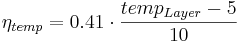
Nitrification and Ammonium Volatilation
The transformation processes of the ammonium pool in this model are the nitrification from ammonium to nitrate and the ammonium volatilation. The calculation of the total transformation of the ammonium pool is carried out for both processes together. Afterwards, the rates for both processes are separated. In order to represent the influence of the temperature, the following coefficient needs to be calculated:
 [1]
[1]
with
 = soil temperature coefficient [-]
 = temperature of the soil layer [°C]
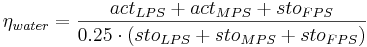
The influence of the soil humidity on the nitrification is described via the coefficient eta_water:
for 
 [2]
[2]
for 
 [3]
[3]
with
 = soil humidity coefficient [-]
 = maximum large pore storage of the horizon [l]
 = maximum middle pore storage of the horizon [l]
= maximum fine pore storage of the horizon [l]
= actual large pore storage of the horizon [l]
 = actual middle pore storage of the horizon [l]
The dependency of the ammonium volatilation on the soil depth is calculated with the following equation:
 = soil depth coefficient [-]
= layer depth of the horizon [cm]
The Gesamtumsatz of the ammonium pool can be calculated as follows:

This Gesamtumsatz is then distributed into:


with
= soil humidity coefficient [-]
= soil temperature coefficient [-]
= soil depth coefficient [-]
 = soil humidity coefficient [kgN/ha]
 = Gesamtumsatz of the ammonium pool [kgN/ha]
 = fraction nitrification [-]
 = fraction ammonium volatilation [-]
 = amount of nitrification [kgN/ha]
 = amount of ammonium volatilation [kgN/ha]
Pre-calculation for the Influence of Environmental Conditions
In order to show the influence of the soil temperature and soil humidity in the different transformation processes, the following coefficients need to be calculated beforehand: U
 [1]
[1]
with
 = soil temperature coefficient [-]
= temperature of the soil layer [°C]
 [2]
[2]
with
 = soil humidity coefficient [-]
= maximum large pore storage of the horizon [l]
= maximum middle pore storage of the horizon [l]
= maximum fine pore storage of the horizon [l]
= actual large pore storage of the horizon [l]
= actual middle pore storage of the horizon [l]
Transfer between the Organic Pools
The transfer between the active and the stable organic pool can be calculated with the following equation:

with
 = transfer rate between the active and stable organic pool [kgN/ha]
 = transfer constant between the active and stable organic pool; default value= 0.00001 [-]
 = active organic pool [kgN/ha]
 = stable organic pool [kgN/ha]
 = fraction of the organic nitrogen in the active organic pool = 0.02 [-]
The transfer rate is here subtracted from the active pool whereas it is added to the stable pool.
Mineralization of the Active Pool
The active pool is mineralized to nitrate directly without taking the nitrification into account. The rate is calculated as follows:

with
 = transfer rate between the active organic and the nitrate pool [kgN/ha]
 = transfer constant between the active organic and the nitrate pool; default value = 0.002 [-]
= active organic pool [kgN/ha]
= soil humidity coefficient [-]
= soil temperature coefficient [-]
The transfer rate is subtracted from the active pool whereas it is added to the nitrate pool.
Dynamics of the Residue Pools
The dynamics of the decomposition of fresh organic substances (residue) from plant remains and organic fertilizer is carried out only in the top horizon. The residue are divided in two pools: the first one represents the biomass as a whole, the second represents the residue's amount of nitrogen. The supply to the residue pools is carried out via plant remains after the harvest and via the organic fertilization with the help of the following equation:


with
 = residue pool [kg/ha]
 = inputted biomass [kg/ha]
 = inputted nitrogen via organic fertilization [kgN/ha]
 = residue pool's amount of nitrogen [kgN/ha]
The decomposition of the residue pool is carried out against the carbon-nitrogen relation (C/N-relation). The calculation of the C/N-relation is carried out according to the following equation.
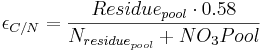
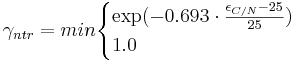
with
 = C/N-relation [-]
 = residue decomposition factor [-]
= residue pool [kg/ha]
= nitrate pool [kgN/ha]
= residue pool's amount of nitrogen [kgN/ha]
The decomposition constant of the residue pool is calculated with γntr, γwater, γtemp:

with
 = constant of the residue decomposition’s rate [-]
= residue decomposition factor [-]
 = residue decomposition coefficient; default value = 0.05 [-]
= soil humidity coefficient [-]
= soil temperature coefficient [-]
The decomposition of the residue pool is carried out with the constant of the residue decomposition’s rate. At this, the nitrogen part is allocated to the active organic pool, in terms of humification, and the nitrate pool, in terms of mineralization, in a ratio of 20:80.


with
= constant of the residue decomposition’s rate [-]
 = residue pool before the time step [kgN/ha]
 = residue pool after the time step [kgN/ha]
 = active organic pool before the time step [kgN/ha]
 = active organic pool after the time step [kgN/ha]
= soil nitrate pool before the time step [kgN/ha]
= soil nitrate pool after the time step [kgN/ha]
 = residue pool's amount of nitrogen before the time step [kgN/ha]
 = residue pool's amount of nitrogen after the time step [kgN/ha]
Denitrification
Denitrification occurs when the soil is nearly water-saturated. The rate depends on the amount of organic carbon in the soil as well as on the soil temperature. In comparison to SWAT (0,95), the degree of water saturation is lower (0.91) when denitrification occurs. This is because SWAT - in contrast to J2000 - does not consider the soil's air capacity. Thus, the underlying pore volume for the calculation of water saturation is higher in J2000. Furthermore, it is ensured that the rate is at the most 1 kgN/ha*d since higher rates are not expected in open land.

with
= soil nitrate pool [kgN/ha]
 = denitrification rate [kgN/ha]
= soil humidity coefficient [-]
= soil temperature coefficient [-]
 = denitrification coefficient; default value = 0.91 [-]
Mass Transport with Water Movement in the Soil
Nitrogen Concentration of Mobile Water
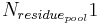
For the simulation of the mass transport caused by water movement, the nitrogen concentration of the mobile water is defined. Here, it is simplified assumed that only the nitrogen of the nitrate pool is mobile and therefore is taken into account for the calculation. The amount of water is determined on the basis of the soil storages and the water streams that leave the horizon.

with
= soil nitrate pool [kgN/ha]
 = soil water [mm]
 = amount of mobile water [mm]
 = percolation coefficient; default value = 0.2 [-]
 = surface runoff [mm]
 = interflow [mm]
 = percolation in deeper horizons or ground water [mm]
 = infiltration water that goes into deeper layers in a time step and therefore passes by the actual horizon [mm]
 = water that leaves the horizon via diffusion [mm]
 = fraction of the pore volume from which anions are excluded (due to positive charge preponderance of the clay mineral); default value = 0.05 [-]
 = nitrogen concentration of the mobile water [kgN/ha*mm]
The influence of the water that expands into deeper horizons in a time step is determined with a parameter ( ). At this, the parameter represents to what extend the bypass water interacts with the soil matrix or bypasses the layers that are flown through in macro pores.
![hor_{by_{infilt}}[i-1] = \sum^{n}_{i}{hor_{by_{infilt}}} * infil_{conc_{factor}} \!](/ilmswiki/uploads/math/2/9/5/29521387268f9a1f06a8919346e9fc41.png)
with
= infiltration water that goes into deeper layers in a time step and therefore passes by the actual horizon [mm]
 = bypass parameter [mm]
= actual horizon [-]
= number of horizons [-]
Nitrogen Transport in the Runoff Components
For the individual horizons the nitrogen loads for the runoff components are calculated on the basis of the mobile water's nitrogen concentration. At this, the interflow is considered in all horizons whereas the surface runoff is only considered in the top horizon. However, the percolation occurs in the deeper horizons or in the ground-water reservoir.


with
= nitrogen concentration of the mobile water [kgN/ha*mm]
= infiltration water that goes in deeper layers and thus bypasses the actual horizon in a time step [mm]
 = nitrogen in the surface runoff [kgN/ha]
 = nitrogen in the interflow [kgN/ha]
 = nitrogen in the percolation water [kgN/ha]
= surface runoff [mm]
= interflow [mm]
= percolation [mm]
 = percolation coefficient [-]
The percolation coefficient represents a measurement for the interaction of the surface runoff and the soil matrix of the top horizon and therefore determines the surface runoff's amount of nitrogen.
The material that leaves the horizon with the diffusion water can be calculated as follows: the water movement that occurs above the field capacity due to potential gradients is called diffusion. Here, a negative value for the diffusion water means a downward water movement whereas a positive value represents an upward water movement.
![diffoutN =
\begin{cases}
w_{l_{diff}}[i] * ConcN_{mobile}[i] & \mathrm{f\ddot{u}r} \; \; w_{l_{diff}} < 0 \\
w_{l_{diff}}[i] * ConcN_{mobile}[i+1] & \mathrm{f\ddot{u}r} \; \; w_{l_{diff}} < 0
\end{cases}](/ilmswiki/uploads/math/5/2/d/52d8953e30a1b04c6d9dd799c9a047e4.png)
and
![NO_3Pool[i] = NO_3Pool[i] + diffoutN \!](/ilmswiki/uploads/math/7/b/5/7b57cb1ca33cde9ac1002c2b7af7788c.png)
and
![NO_3Pool[i+1] = NO_3Pool[i+1] - diffoutN \!](/ilmswiki/uploads/math/8/d/a/8da310efcecc92e2ec1b314ec8d885d8.png)
with
= nitrogen concentration of the mobile water [kgN/ha*mm]
 = nitrogen in the diffusion water [kgN/ha]
= soil nitrate pool [kgN/ha]
 = diffusion water [mm]
= soil horizon [kgN/ha]
Soil Temperature Module
The soil temperature is an important measurement for the matter regime modeling. Especially microbiological processes such as nitrification, denitrification and the transformation of organic nitrogen in the soil zone is strongly influenced by the prevailing temperature. In the here developed model J2K-S the soil temperature also plays an important role for the calculation of the following processes (see Soil Nitrogen Module):
• nitrification
• volatilation
• transformation of organic substance
• decomposition of plant remains
• denitrification
Structure of the Module
The soil temperature is simulated according to the empirical routines of SWAT (Arnold et al. 1998) and EPIC (Williams et al. 1984). At first, a surface soil temperature is generated for bare ground on the basis of the air temperature and insolation. This surface temperature is modified by attenuation factors that describe the effect of biomass and snow. The temperature of the different soil horizons is generated as upper boundary condition between the surface soil temperature and the long lasting mean temperature as lower boundary condition. At this, the attenuation effect of the soil is defined in consideration of the soil humidity and the bulk density. The equations of the individual processes can be found in Neitsch et al. (2002).
Figure 1: Structure of the soil temperature model
Figure 2: Results of the soil temperature modeling for the surface area and at 40 cm depth at an investigated slope near Zeulenroda (Thuringia).
This figure shows the measured and modeled temperature at the surface (upper figure) as well as at 40 cm depth (lower figure) for an investigated area near the dam Zeulenroda. It can be seen that the temperature curve can be followed quite well in spite of certain deviations. This is emphasized by the high coefficient of determination of about 0.95.
Plant Growth Module
The description for the simulation of plant growth is important for numerous hydrological mass transport processes, e.g. for the interception or the nitrogen uptake by the canopy. Plant growth is usually controlled via the simulation of the leaf area development (LAI) as well as the light interception and the transformation into biomass and is carried out according to SWAT (Arnold et al. 1998). At this, it is assumed that a potential plant growth, i.e. under optimum conditions, exists which is then modified in consideration of stress factors.
Temperature Development and Heat Units
The most important factor that determines the canopy’s development is the temperature whose parameters are different for each plant. Therefore, each plant possesses a basis temperature that needs to be reached in order to activate a certain growth. The growth increases until the optimum temperature is reached and decreases noticeably when the maximum temperature is exceeded. The plant-specific growth development is carried out via the generating of heat units (=HU). The underlying hypothesis for this is the assumption that plants have a specific heat demand that is quantifiable until the necessary maturity state for the harvest is reached. An ‘HU’ is defined as a phenological effective temperature unit. An HU results from the daily accumulated daily average temperature that lies above the plant-specific basis temperature. Assumed that a maize plant has a basis temperature of 7° C and is exposed to a daily temperature of 15° C, its HU would be calculated as follows: 15 – 7 = 8 HUs. In this way, the individual heat unit developments are simulated for each land use type in consideration of the time of the sowing and harvest as well as the daily average temperature. The development of the root growth and the leaf area index is controlled via the heat unit development. At this, it is assumed that the plants invest their energy into the leaf development and the root growth. This simplified view also means that the development of leafs and roots is independent on water and nutrient supply. Furthermore, the plant’s degree of maturity which influences the amount of nitrogen in the biomass is exclusively controlled via the temperature sum.
Biomass Development
The biomass development is simulated as potential biomass at first. At this, the photosyntetic radiation is the controlling unit for the biomass development. Thus, a potential biomass increase is generated for each day with the help of the radiation and leaf area (see figure 1).

Figure 1: Structure of the plant growth module
This daily biomass increase is reduced to the actual biomass increase with the help of stress factors, which are nitrogen supply, temperature and water supply (see figure 2).

Figure 2: Structure of the growth’s stress
The stress factor that has the strongest effects at a point in space and time determines the actual biomass according to the principle of limiting factors. This, in turn, influences the nitrogen demand.
Land Use Management Module
The description of the land use management is carried out according to the methodology in the SWAT model (Arnold et al. 1998). The land use management module offers to represent complex crop rotations in J2k-S. The individual field crops are characterized on the basis of management operations like sowing, fertilizing and harvesting. As can be seen in figure 1, the crop rotation relates to an actual plant that in turn is build up of the plant parameters and the individual management options.
Bild:Pflanzenmanagementmodul1.jpg
Figure 1: Flow chart of the land use management module
The basic basis objects for the description of the land use management are cultivation (no function yet), fertilization, plant characteristics and the crop rotation. Land management and fertilization as management options have only simple parameters like mixing efficiency, machining depth, amount of fertilizer, ammonium and nitrate. However, the plant object possesses numerous parameters. Thus, the crop rotation is a simple list with the order of the individual crops (see figure 2).
Bild:Pflanzenmanagementmodul2.jpg
Figure 2: Essential components (basic objects)
As an explanation in figure 3 a detail of a management parameter file is shown. In the first line a cultivation type can be found. Thereupon, the sowing of the maize that was used in the example follows. Furthermore, three fertilizations with three different fertilizers are carried out. The harvest with the amount of biomass is given. The rest remains on the field and is allocated to the residue pool in the nitrogen module. Finally, cultivation is carried out in this example.
Bild:Pflanzenwaschtumsmodul4.jpg
Figure 3: Structure of a management parameter file
With the help of this tool, the essential activities of the horticultural management as well as alternatives can be represented flexibly.
Ground Water Nitrogen Module
The description of the nitrogen’s dynamics that occurs in the ground water is carried out according to the ground water dynamics used in J2k. At this, the nitrogen load is – corresponding to the water – allocated to the two ground-water reservoirs RG1 and RG2. The water and matter proportions are generated for both ground-water reservoirs. The output is carried out analogue to the water and the generated proportions. It is possible to set up an origin nitrogen concentration.
Besides, an attenuation factor is implemented that delays the change of the nitrogen proportions in the storage. This factor used for the calibration can be set up for both ground-water reservoirs separately. It represents the mixing and diffusion effects in the aquifer.
Back to Models