Tutorial Calibration
Contents |
Motivation
In order to apply hydrological models successfully it is necessary to define model parameters accurately. A direct measurement of the parameters is mostly not possible, too expensive or there is no clear physical relation. For those reasons the parameters are adjusted in a trial and error process in so far that the simulated factors (e.g. runoff) correspond best to the values measured. This task can be time-consuming and difficult if the corresponding model is complex or has a large number of parameters.
Requirements
The callibration of the model has multiple requirements:
- the model must be executable.
- there must be at last one measured/observed timeline that can be compared with the model results.
- an evaluation criteria must be calculated for the quantification. The calculation should be done with the UniversalEfficiencyCalculator. You can find an tutorial for adding those components here.
Calibration
There are two common methods for calibrating a model with the integrated Standard Efficiency Calculator:
Offline Calibration
First, it is possible to carry out a calibration locally on your own computer. However, this uses computing resources for a longer period of time. Step 1
Open the JAMS User Interface Model Editor (JUICE).
Load the model you want to calibrate.
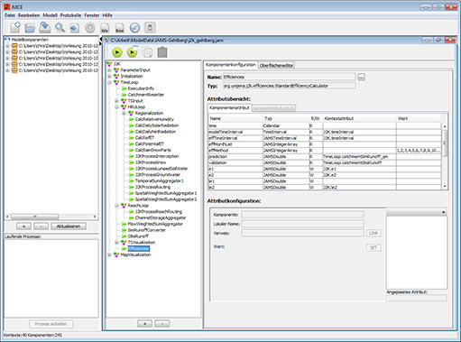
The following window should appear:
Step 2
Select the entry Kalibrierungswizard under the item Modell.
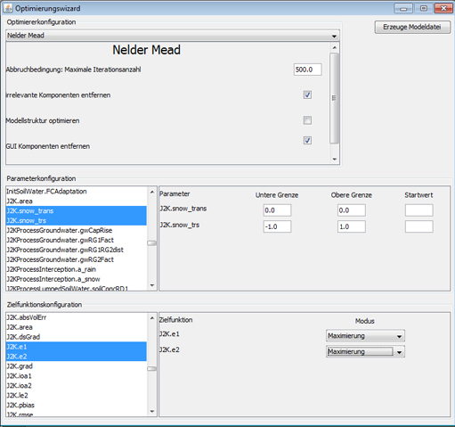
A dialog should appear which offers the configuration of the calibration (see image).
Step 3
In the middle of the dialog area on the left hand side the potential parameters of the model are listed. Select those parameters from the list which you want to calibrate. If you want to select more than one parameter, hold down CTRL while selecting the parameters. Now you can see several input fields for each parameter on the right hand side. You can choose the lower and upper bound which define the area in which the parameter can vary. In addition, it is possible to define a start value. This makes sense if a parameter is already known which suits as a starting point for the calibration.
Step 4
In the the lower area in the dialog the target function is specified. Either a single criterion or various criteria can be selected (for more than one hold CTRL). By choosing various criteria a multi-criteria optimization problem is created which differs significantly from a (common) one-criterion optimization problem regarding its solution. Since not every optimization method is suitable for a multi-criteria problems either, not all optimizers are at disposal this time.
For every selected optimization criterion a list box appears on the right hand side of this section. It determines whether the criterion will be minimized, maximized, absolutely minimized (i.e. min |f(x)| e.g. for the absolute volume error) or absolutely maximized.
Step 5
When parameters and target criteria are selected, it is necessary to choose an optimization method for the calibration. In the upper area of the dialog you can see a list box which lists several optimization methods. At the moment the following methods are available:
- Shuffled Complex Evolution
- Branch and Bound
- Nelder Mead
- DIRECT
- Gutmann Method
- Random Sampling
- Latin Hypercube Random Sampler
- Gauß Process Optimizer
- NSGA-2
- MOCOM
- Paralleled Random Sampler
- Paralleled SCE
For the application with single target criterion the Shuffled Complex Evolution (SCE) and DIRECT are recommended. Most probably both find a global optimized parameterization. It has been attested that DIRECT shows robust operation and no parameterization is necessary. SCE only needs one parameter: the Anzahl der Komplexe (number of complexes). This parameter indirectly controls whether the parameter search area is browsed rather broadly or if the process quickly concentrates on a (sometimes local) minimum. In most cases, the default value 2 can be used. For multi-criteria optimization NSGA - 2 seems to provide very good results. However, there are more detailed analyses to be carried out.
In addition, there are three check boxes available, independent of the selected method.
- irrelevante Komponenten entfernen: deletes components from the model structure which certainly do not influence the calibration criterion
- GUI Komponenten entfernen: deletes all graphical components from the model structure. This option is strongly recommended since e.g. diagrams have a strong negative influence on the calibration.
- Modellstruktur optimieren: at the moment without function
Step 6
In order to finish the configuration, click on the button XML erzeugen. This closes the dialog and a new (modified) model is set up. You can start the calibration by starting the modeling. Please keep in mind that the calibration assistant modifies your output data stores in such a way that for every model run during calibration model parameters and target criteria are given. If you want to avoid this output, delete the file optimization_wizard_optimizer.xml manually.
Online Calibration
As an alternative to offline calibration the process can be carried out on the computing cluster of the Department of Geoinformatics, Hydrology and Modelling at the Friedrich - Schiller - University Jena. This does not occupy any local computing resources and allows a calibration of up to four models at the same time.
Step 1
Open your Internet browser (e.g. Firefox) and go to website [[1]] You will now see the following window and you will require a login. In order to register please contact
- Christian Fischer
- christian.fischer.2@uni-jena.de
Step 2
After the registration you will see the main window of the application.
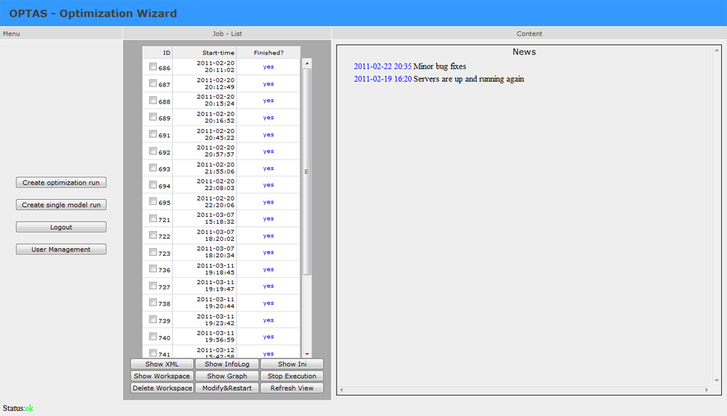
The window is split up into three parts. In the middle you can see a list of all tasks that have been started. All tasks which have been finished are marked in blue color and tasks which are being carried out are marked green. Red entries indicate that an error has occurred during the configuration of a new task/calibration. The right part of the window shows different contents. When starting the application, you can see news about the OPTAS project. In general, information up to a size of 1 megabyte is shown. Greater data sizes are not shown because it affects the page view. Instead, a zip file is created from the information which is then available for download.
Step 3
In order to carry out a new calibration, click on "Create Optimization Run". You will now see the first step of the calibration process.

In this step you will be asked to enter the data which is necessary. Load the model for the calibration (jam file) into the first file dialog. Pack your working directory of the model as a zip archive. A suitable programs is for example 7-zip. Please note:
- the working directory cannot be in a subfolder
- please do not load any unnecessary files (e.g. in the output file). The upload is limited to 20mb.
- the file default.jap is not allowed to be in the working directory
Now load the packed working directory into the second file dialog. The modeling will usually be carried out by using the current version of JAMS/J2000. Libraries for J2000g and J2000-S are usually available as well, so you will not need any files for most applications.
Should you need any versions of component libraries which are particularly adapted for models J2000, J2000-S or J2000g, please load them (unpacked) into the corresponding file dialogs. If your models requires additional libraries, you can indicate them as a zip archive in the corresponding file dialog.
To finish, click on Submit. The files that you indicated are now are now being loaded on the server environment.
The management server (sun) checks the host for free capacities and assigns a host to your Task.
Step 4
After transferring the model and the workspace, the following dialog for the selection of parameters and goal criteria appears.
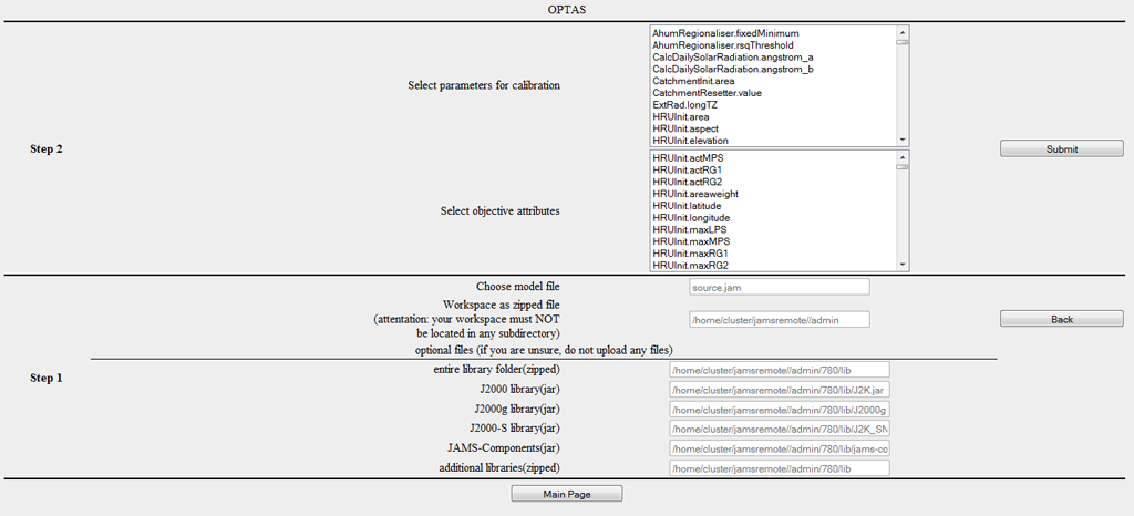
The first list shows all potential parameters of the model. Select those parameters which you want to calibrate. If you want to select several parameters, hold CTRL when marking them.
In the low part of the dialog a target function is specified. You can either select a single criterion or several criteria (hold CTRL). When selecting several criteria, a multi-criteria optimization problem is created which differs significantly from a (common) one-criteria optimization problem regarding its solution characteristics. Since not every optimization method is suitable for multi-criteria problems, not all optimizers are available in this case.
Step 5
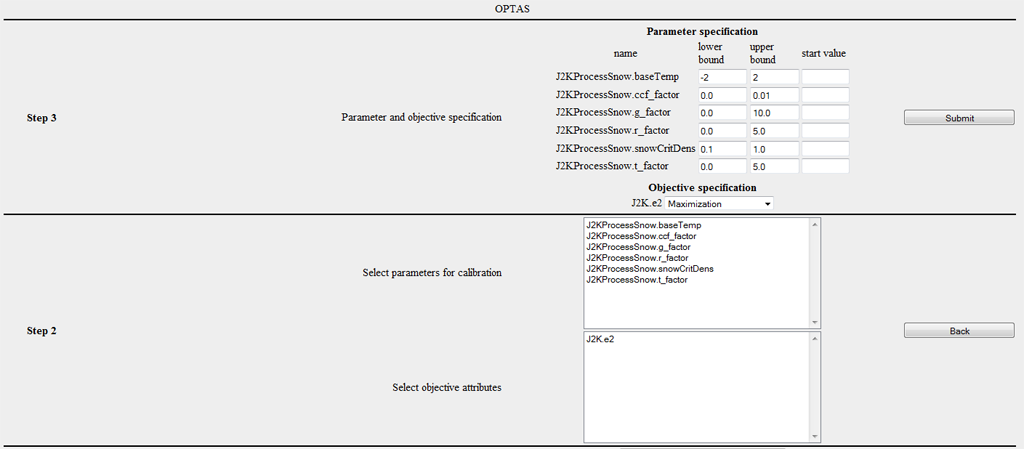
In this step, the valid range of values is to be specified for every parameter. For every selected parameter an input field is available for the specification for upper and lower boundaries. The fields are occupied by default values, if they are available for the specific parameter. These default values are mostly very broad, so it is recommended to carry out further restrictions. In addition, there is an optional possibility to indicate the start value. This is helpful if an adequate set of parameters is already available which is taken as the starting point of the calibration.
In the second part, you can choose for every criterion whether it should be
- minimized (example RSME - root square mean error),
- maximized (example r²,E1,E2,logE1,logE2),
- absolutely minimized (i.e. min |f(x)| e.g. for absolute volume error),
- or absolutely maximized.
The following image shows the corresponding dialog. In this example, the parameters of the snow module were chosen and the default thresholds were entered.
Step 6
You are now asked to choose the desired optimization method. At the moment, the following methods are available:
- Shuffled Complex Evolution (Duan et al., 1992)
- Branch and Bound (Horst et al., 2000)
- Nelder Mead
- DIRECT (Finkel, D., 2003)
- Gutmann Method (Gutmann .. ?)
- Random Sampling
- Latin Hypercube Random Sampler
- Gaußprozessoptimierer
- NSGA-2 (Deb et al., ?)
- MOCOM ()
- Paralleled random sampling
- Paralleled SCE
For most one-criterion applications the Shuffled Complex Evolution (SCE) method and the DIRECT method can be recommended. For multi-criteria tasks the NSGA-2 mostly delivers excellent results.
Step 7
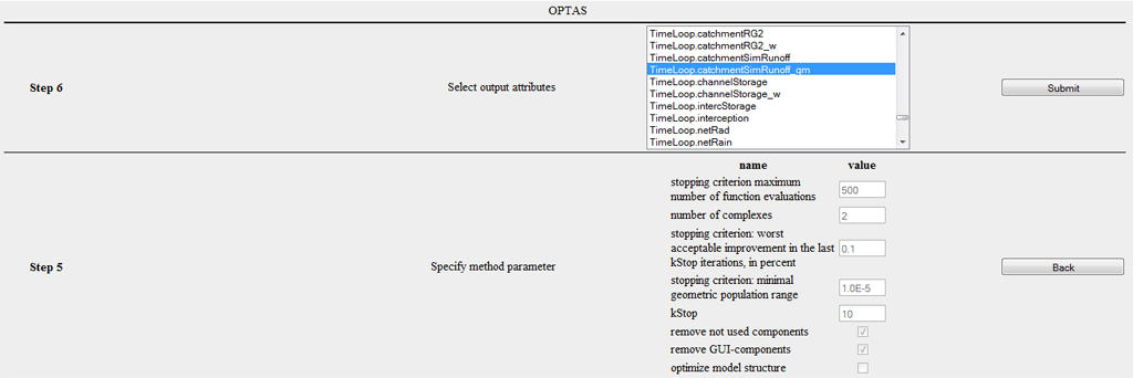
Many optimizers can be parametrized according to the specific task. SCE has a freely selectable parameter: the number of complexes. A small value leads to rapid convergence, though with higher risk of not identifying the global solution, whereas a greater value increases calculation time significantly while strongly improving the possibility of finding an optimum. Mostly a default value of 2 can be used to work with. In contrast, DIRECT for example does not possess any parameters. It shows a very robust behavior and no parametrization of the method is required. Moreover, three check boxes are available which are not subject to the specific method.
- remove not used components: removes components from the model structure which definitely do not influence the calibration criterion
- remove GUI-components: removes all graphical components from the model structure. This option is highly recommended since e.g. diagrams influence the efficiency of the calibration in a very negative way
- optimize model structure: at the moment without function
The following image shows step 7 for the configuration of the SCE method.
Step 8
Before starting the optimization you can indicate which variables/attributes of the model should appear in the output. As a default, those parameters and target criteria are shown which have already been chosen which makes manual selection unnecessary. Pleas note that saving temporally and spatially varying attributes (z.B. outRD1 für jede HRU) may require a huge amount and this may exceed the size belonging to a user account.
Step 9
You now receive a summary of all modifications which have been carried out automatically. Particularly, you now have a list of components which are classified as irrelevant. By clicking on Submit you start the optimization process.
Operating OPTAS
After having started the calibration of the model, you should now see a new job on the main page. This is shown green to indicate that the execution is not yet completed. You also see the ID, the start date and the estimated date of completion for the optimization. If you select the generated job, you now have various options at your disposal.
Show XML
You can see the model description for carrying out this job which has automatically been generated. As soon as you click on the button, it appears on the right hand side in the window and can be downloaded from there as well.
Show Infolog
Click on this button in order to view status messages of the current model. When using an offline execution of the model this information is written in the file info.log or error.log.
Show Ini
The optimization-Ini file contains all settings applied and summarizes them in abbreviated form. This function is meant for the advanced user or developer, hence there is no further explanation at this place.
Show Workspace
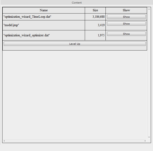
This function lists all files and directories in the workspace. By clicking on the directory/file its content is shown. The modeling results can usually be found in the file /current/ which is shown as an example in the following image.
It is to be noted that file contents can only be represented up to a maximum size of 1 megabyte and they are otherwise zipped in a zip file and made available for download.
Show Graph
Dependencies between different JAMS components of a model can be graphically displayed. This function generates a directed graph the node of which is the number of all components in the model. In this graph, a component A is linked to a component B if A is dependent on B, in the sense that B generates data which are directly required from A. Moreover, all components are shown red which have been deleted during model configuration. This dependency graph allows for an analysis of complex dependency relations, as for example the determination of components which are indirectly dependent on a certain parameter. Such kinds of analyses should, however, not be carried out. The graphical output of this graph is primarily used for visualization.
Stop Execution
Stops the execution of one or more model runs.
Delete Workspace Deletes the complete workspace of the model on the server environment. Please use this function when the optimization is completed and when you have saved the data. This discharges the server environment and accelerates the display of the OPTAS environment.
Modify & Restart This function is addressed to advanced users. Often a restart of a model or calibration task is required without further need of modifications in the configuration. By using the function Modify & Restart the configuration file of the optimization can be directly changed and afterwards the restart of the model can be enforced in a new workspace.
Refresh View Updates the view. Please do not use the update function of your browser (usually F5) since this leads to a re-execution of the last command (e.g. starting the model).
Model Validation
The model validation serves as evidence for the suitability of a model for a certain intended purpose (Bratley et al. 1987). Model validation is an important tool for quality assurance. A model is useful for implementation if it proves to be a reliable representation of real processes (Power 1993). Different key figures and proofs may be required subject to the purpose and type of model in order to validate the model.
In general, there are different quality criteria which play a role for model validation:
- Accuracy/precision: The accuracy of a model represents the deviation of simulated values in comparison to real (measurement) values. This is mostly quantified by the Nash-Sutcliffe efficiency, degree of determination or mean square error.
- Uncertainty: The input values of an environmental model often contain errors and uncertainties. In addition, there is no complete knowledge regarding a natural system, i.e. the modeling has uncertainties. The impact of these values is quantified by the insecurity of the model, i.e. the uncertainty reveals the confidence interval of a model response.
- Ruggedness: The ability of the model to maintain its function if there are (minor) changes in the natural system (e.g. change of land use in a catchment area). This is closely linked to
- Sensitivity: which indicates the influence of (minor) changes in the input data and model parameters on the result
- Validity: is the property of the model to provide correct results for the right reasons, i.e. the explanation for a system which is given by the model is correct.
The following methods for the validation of hydrological models were put forward by Klemes (1986).
Split Sample Validation
The amount of validation data which is available (e.g. runoff time scales) is split into two sections. First, section 1 is used for calibration and section 2 for validation of the model. Then the calibration part and the validation part are swapped. For this reason both section should have an equal size and provide a for adequate calibration. The model can be classified as acceptable if both validation results are similar and have sufficient properties for model application. If the available amount of data is not large enough for a 50/50 division, the data should be split in such a way that one segmaent is large enough to carry out a reasonable calibration. The part remaining is used for the validation. In this case the validation is supposed to be carried out in two different ways. For example, (a) the first 70% of the data are used for calibration and the remaining 30% for validation, (b) then the last 70% of the data for calibration and the remaining first 30% for validation.
Cross Validation
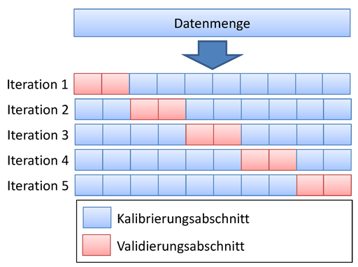
Cross validation is a further development of the split sample test. The amount of data is split up into n sections of equal size. Now n − 1 sections are used for the calibration and the remaining part is used for validation. The amount for the validation is swapped, so every set of data is validated once. This method requires much more computational effort than the split sample validation but it has major advantages if there is a small amount of data and it allows for a validation of every kind of data set. A special case of this validation is the Leave-One-Out Validation (LOO). It always uses exactly one data set for validation and the remaining part for validation. Due to the huge effort this kind of validation is mostly applied in special cases.
Proxy Basin Test
This is a basic test concerning the spatial transferability of a model. If, for example, the runoff is supposed to be simulated for a non-measured area C, two measured areas A and B can be selected within a region. The model should be calibrated with data from area A and validated using data from area B. Then roles of area A and B should be exchanged. Only if both validation results are acceptable with regard to modeling application, it can basically be assumed that the model is able to simulate the runoff of area C. This test should also be applied if an amount of data is available for area C which is not sufficient for the split sample test. The data set in area C would not be used for mode development but only as an additional validation.
Differential Split-Sample Test
This test should always be used if a model is supposed to be applied under new conditions in a measured area. The test may have several variants, subject to the way in which the conditions/properties of the area have changed. Those changes include, for example, climate changes, changes of land use, the construction of building, which influence the hydrology in the region etc.
For the simulation of effects of climate change the test should have the following form. Two time periods with different climate parameters should be identified in historical data sets; for example, a time period of high mean precipitation and another period of low precipitation. If the model is supposed to be used for runoff simulation of humid climate scenarios, the model should be calibrated with the arid data set and the validation should be carried out with the "humid" data set. If it is supposed to be used for the simulation of an arid scenario, the procedure should be reversed. In general, the validation is supposed to test the model under changed conditions. If no sections with significantly different climatic parameters can be identified in historical data, the model should be tested in another area where the differential split-sample test can be carried out. This is mostly the case if not climate changes but, for instance, changes of land use are considered. In this case a measured area has to be identified where similar changes of land use have taken place. The calibration should be carried out using original land use and validation using the new land use.
If alternative areas are used, at least two areas of such kind should be identified. The model is calibrated and validated for both areas. The validation can only be successful if results for both areas are similar. It has to be noted that the differential split-sample test, in contrast to the proxy - basin - test, is carried out for both areas independently.
Proxy-basin Differential Split-Sample Test
As the name suggests, this test is a combination of proxy-basin and differential split-sample test and it should be used if a model should be transferable in space and is applied under changed conditions.


