Tutorial Basic Users
System Requirements, Download and Installation of JAMS/J2000
System Requirements
To run JAMS the Java Runtime Environment (JRE) Version 5.0 or higher is required. The installation file can be downloaded here: http://java.sun.com/javase/downloads/index.jsp.
JAMS/J2000 Download
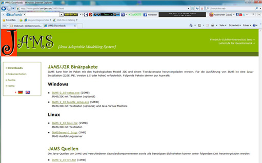
JAMS is available to download at http://www.geoinf.uni-jena.de/5580.0.html as a package including the hydrological model J2000 and a test data set. To run JAMS an installation of Java (J2SE JRE, Version 1.5 or higher) is required.
In addition, all Java sources of JAMS, different standard components as well as all libraries needed are available on this website.
There are packages for Windows and Linux at disposal. If your operating system does not have a Java installation, JAMS/J2000 can be downloaded with a Java Virtual Machine.
The installation for Windows is carried out by an executable file which installs JAMS completely. For Linux a tgz-archive is available which includes all files needed. For the execution of JAMS on Linux an existing Java installation is required.
The installation of JAMS includes two executable files:
- jams.exe (jams on Linux) launches the JAMS-Launcher
- juice.exe (juice on Linux) launches the graphical model editor JUICE
JAMS/J2000 Installation on Windows
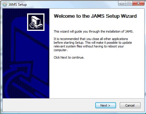
The installation program opens.
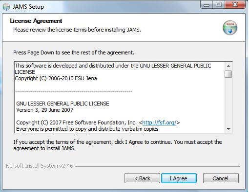
Click on Next and accept the license agreement.
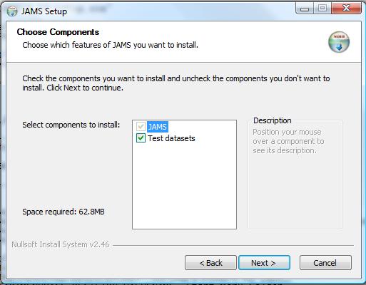
In the next step you can decide whether you would like to install two test data sets in addition to JAMS/J2000. In each of those data sets you can find an example of a model description and all necessary input data for the catchment area.
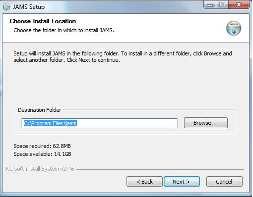
Please select the folder where the program will be installed.
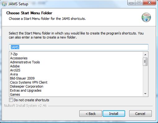
Please select a folder of the start menu to create shortcuts for JAMS Builder, JAMS Launcher, JAMS Remonte Launcher and test data sets.
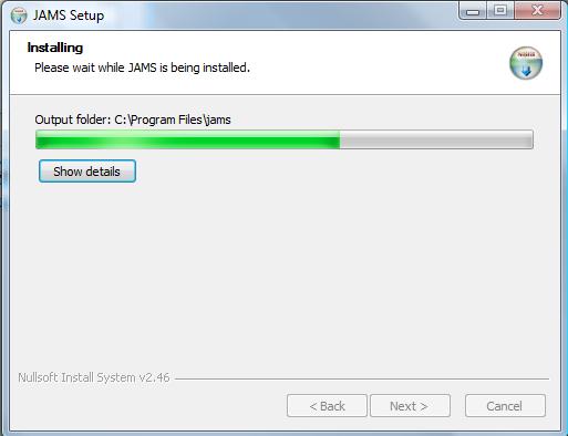
Click on Install to start the installation.
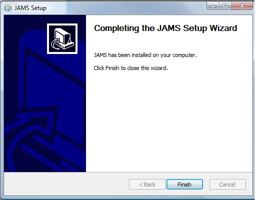
JAMS/J2000 has been successfully installed.
Introduction and Application of the JAMS Launcher
The JAMS Launcher is a graphical surface for editing model configurations and system configurations and a device for model execution. The design is dependent on the model configuration which is currently loaded. Automatically generated input components can serve to define initialization values for specific model parameters.
The JAMS launcher also enables loading and saving model and system configurations. It is automatically displayed when starting JAMS, providing that the feature "guiconfig" has the value "1" in the system configuration.
Structure and Capacity of the JAMS Launcher
The JAMS Launcher is a software tool which facilitates loading and parameterizing models as well as carrying out modelings. Additionally, modeling results can be visualized. The total runoff at the catchment outlet, soil water, snow water equivalent and the map of the catchment area can be examined.
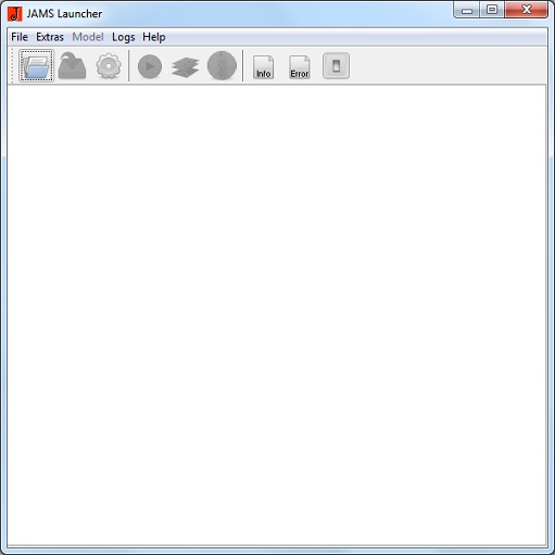
You can start the launcher from the start menu or from a shortcut on your desktop. The following splash screen will appear:
The JAMS Launcher has been opened and can now start the modeling.
Under the menu item File you can load, save and close models.
The menu item Extras can change settings, load and save settings or continue an interrupted model execution.
Under JAMS settings you can change libraries, output size, output of model protocols and information on model windows. Those settings can be saved for later modelings under Edit Preferences and can be loaded under Load Preferences.
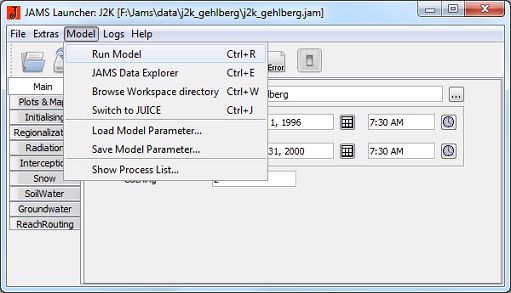
Under the menu item Model, you can start the modeling (Run Model), you can see the current workspace (Browse Workspace directory) or you can see the docket of all ongoing processes (Show Process List).
Under the menu item JAMS Data Explorer you can export the modeling results as well as the input data which are at disposal for the model into the tool JADE. This allows an intensive evaluation of results and an analysis of the measured data used for the modeling.
The menu items Load Model Parameter and Save Model Parameter are used to manage model parameters. An edited parameter set can be saved to reuse it for new modelings.
Under the menu item Logs you can look at the Info Log. It contains information on the model's author, its version or on its user as well as information on the model's efficiency (How well did the model display the measured data?), the model structure (Which components were used and how often?) and on the model runtime.
The Error Log records any errors which may have occurred.
Under the menu item Help you can obtain online help of JAMS by clicking on JAMS online.
Selecting and Running a Model
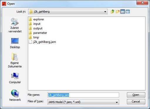
If you want to run a model, select a model description in the JAMS Launcher under the item load file/model. Models can be read as *.xml or *.jam files. If you named the installation folder jams and installed a test data set when installing JAMS, then you will find an example of a model description (j2k_gehlberg.jam) in folder jams/data.
You can start the modeling by clicking on the green button in the menu bar.
Editing Model Parameters
Basic Settings
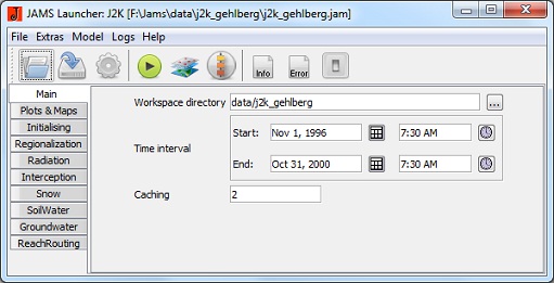
- Workspace directory: Sets the working directory. It has to contain three more folders: Parameter (for all parameter files), Data (for all data files) and Output (for all output files).
- Time interval: The time interval for the model run is selected.
- Caching: The results of some compute-intensive processes can be temporarily stored in hard disk and reused for further model runs. Therefore the model run is slightly faster. Attention: This feature is not completely safe yet and should only be applied by experienced users.
Diagrams and Maps
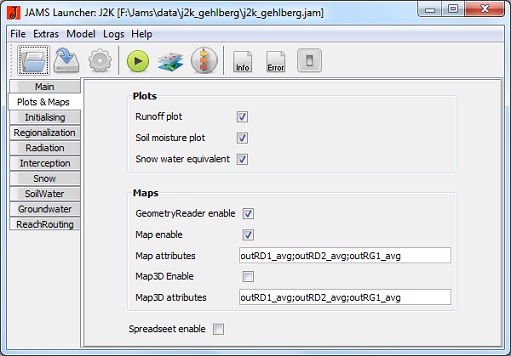
- Runoff plot: Activates the graphical display of the runoff modeled and measured during model run.
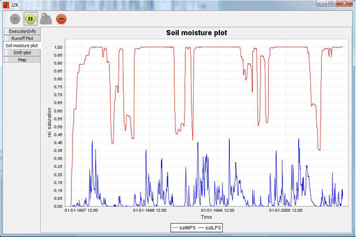
- Soil moisture plot: Activates the graphical display of the relative soil moisture during model run.
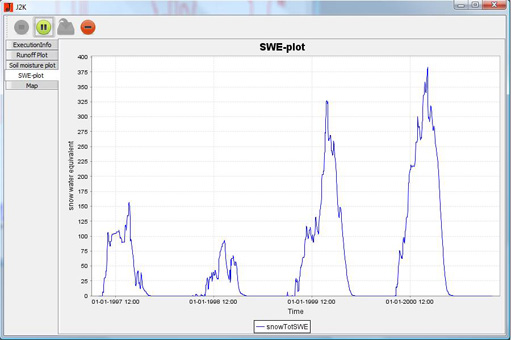
- Snow water equivalent: Activates the graphical display of the snow water equivalent during model run.
- Map enable: Enables the output of a cartographic display of selected state variables.
- Map attributes: A semicolon-separated list of state variables which are to be cartographically displayed.
- Map3D enable: Enables a 3D output of a cartographic display of selected state variables.
- Map3D attributes: A semicolon-separated list of state variables which are to be cartographically displayed (in 3D).
Initialising
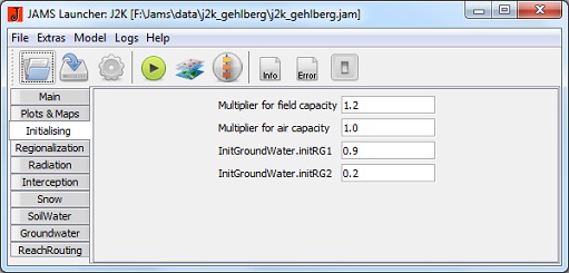
- Multiplier for field capacity : The maximum storage capacity of the middle pore storages (MPS) can be increased (value > 1) or decreased (value < 1).
- Multiplier for air capacity: The maximum storage capacity of the large pore storages (LPS) can be increased (value > 1) or decreased (value < 1).
- initRG1: relative filling of the upper groundwater storage at beginning of model run (1 filled to capacity, 0 empty).
- initRG2: relative filling of the lower groundwater storage at beginning of model run (1 filled to capacity, 0 empty).
Regionalization
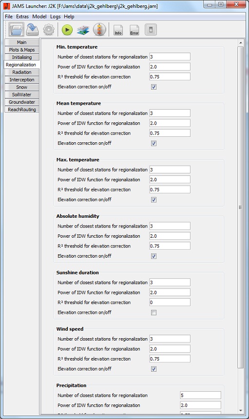
- number of closest stations for regionalization: Number n of stations used to calculate the value of an HRU (n stations which are closest to the HRU are selected).
- Power of IDW function for regionalization: Weighting factor used to exponentiate the distance of each station to the respective HRU.
- elevation correction on/off: Activates the elevation correction of the data values.
- r-sqrt threshold for elevation correction: Threshold value for the elevation correction of the data values. If the coefficient of determination of the regression relation between measured data of the stations and station elevations is smaller than this value, an elevation correction is not carried out.
Those settings (i.e. minimum temperature, maximum temperature, medium air temperature, precipitation, absolute air moisture, wind speed, sunshine duration) can be adjusted for every single input variable.
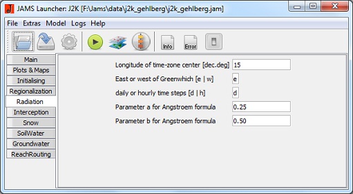
Radiation
- flowRouteTA [h]: runtime of the outflow route
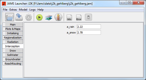
Interception
- a_rain [mm]: Maximum storage capacity of the interception storage per m2 leaf area for rain
- a_snow [mm]: Maximum storage capacity of the interception storage per m2 leaf area for snow
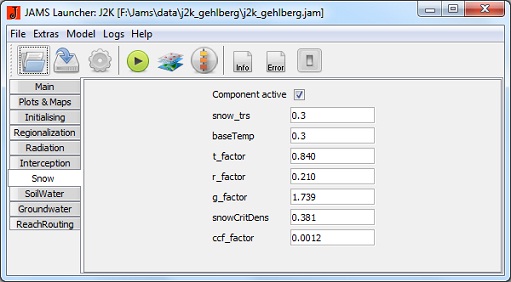
Snow
- Component active: Activates the snow module.
- baseTemp [°C]: Temperature limit value for snow precipitation.
- t_factor [mm/°C]: Temperature factor for calculation of snowmelt runoff.
- r_factor [mm/°C]: Rain factor for calculation of snowmelt runoff.
- g_factor [mm]: Soil heat flux factor for calculation of snowmelt runoff.
- snowCritDens [g/cm³]: critical snow density
- ccf_factor [-]: factor for calculation of the cold content of snow cover
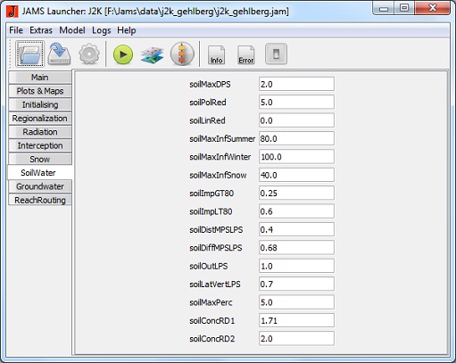
Soilwater
- MaxDPS [mm]: maximum hollow reserve
- PolRed [-]: polynomial reduction factor for reduction of potential evaporation with limited water supply.
- LinRed [-]: linear reduction factor for reduction of potential evaporation with limited water supply.
(Note: PolRed and LinRed do not represent alternatives. Only one can be attributed a value, the other one has to be 0.)
- MaxInfSummer [mm]: maximum infiltration during summer period
- MaxInfWinter [mm]: maximum infiltration during winter period
- MaxInfSnow [mm]: maximum infiltration with snow cover
- ImpGT80 [-]: relative infiltration capacity of areas with a sealing degree of > 80%
- ImpLT80 [-]: relative infiltration capacity of areas with a sealing degree of < 80%
- DistMPSLPS [-]: calibration coefficient for distribution of infiltration on soil storages LPS and MPS
- DiffMPSLPS [-]: calibration coefficient for the definition of the diffusion amount of the LPS storage in relation to MPS at the end of a time step
- OutLPS [-]: calibration coefficient for definition of LPS outflow
- LatVertLPS [-]: calibration coefficient for distribution of the LPS outflow on the lateral (interflow) and vertical (percolation) component
- MaxPerc [mm]: maximum percolation rate
- ConcRD1 [-]: retention coefficient for direct runoff
- ConcRD2 [-]: retention coefficient for interflow
Groundwater
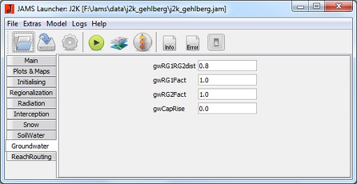
- RG1RG2dist [-]: calibration coefficient for distribution of percolation water
- RG1Fact [-]: factor for runoff dynamics of RG1
- RG2Fact [-]: factor for runoff dynamics of RG2
- CapRise [-]: factor for the setting of capillary rise
Routing in the Flow
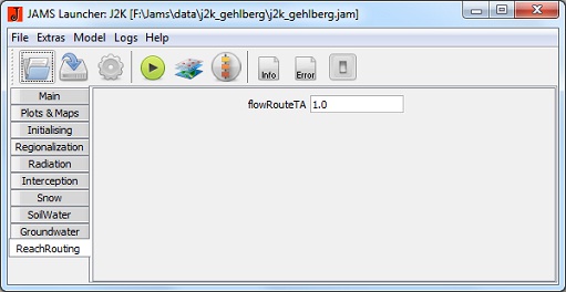
- flowRouteTA [h]: runtime of the outflow route
Visualization of Modeling Results
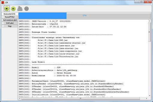
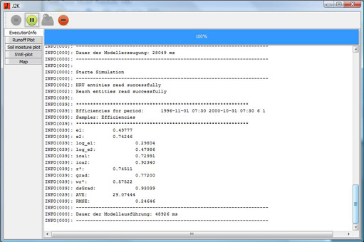
After the modeling has been successfully carried out, the following window opens automatically:
The ExeptionInfo contains information on the model's author, its version or on its user as well as information on the model's efficiency (How well did the model display the meadured data?), the model structure (Which components were used and how often?) and on the model runtime.
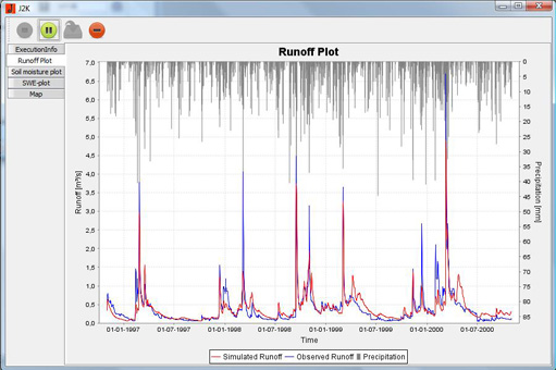
The Runoff Plot can compare the simulated runoff with the runoff actually measured. The precipitation is shown in this diagram as well.
The SWE Plot contains information on how much water is stored as snow.
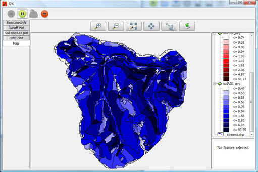
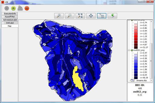
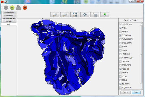
Under the menu item Map the catchment area is shown with its modeling units. In the right window all those variables are listed which were selected in the JAMS Launcher/Plots & Maps/Map attributes. They can be evaluated in different maps.
The value of a single modeling unit variable can be shown by clicking on the modeling unit.
The map can be exported with selected attributes as *.shp.
Application of the JAMS Data Explorer (JADE) for Result Analysis
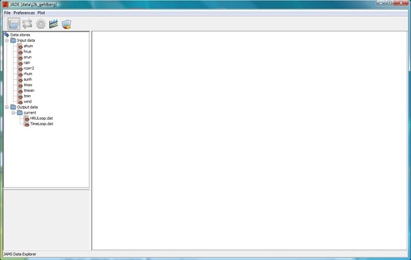
By using the JAMS Data Explorer (JADE), on the one hand, input data which were the basis for the modeling can be displayed. On the other hand, the JADE tool can evaluate and visualize calculated output data. The JADE can be launched under the menu item Modelle/JAMS Data Explorer. The input data which were the basis for the modeling are automatically loaded (Input data). Moreover, the output folder generated during the modeling will be loaded (Output data). In this way, all modeled data can be loaded, displayed and analyzed.
Analysis of Input Data for the Modeling
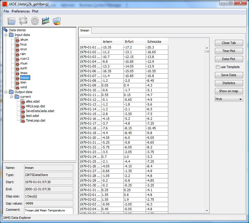
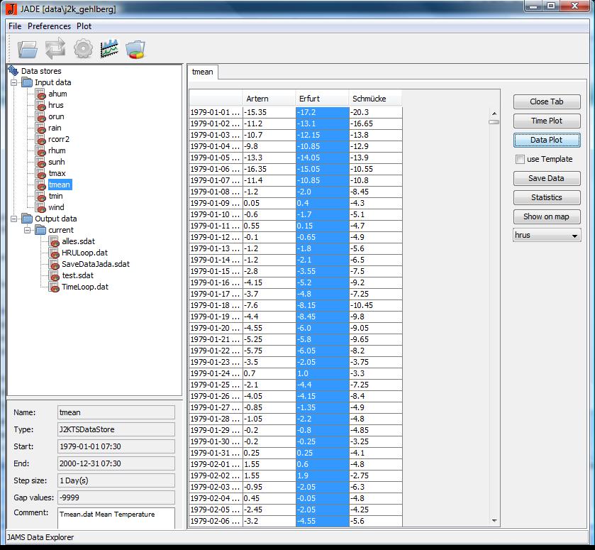
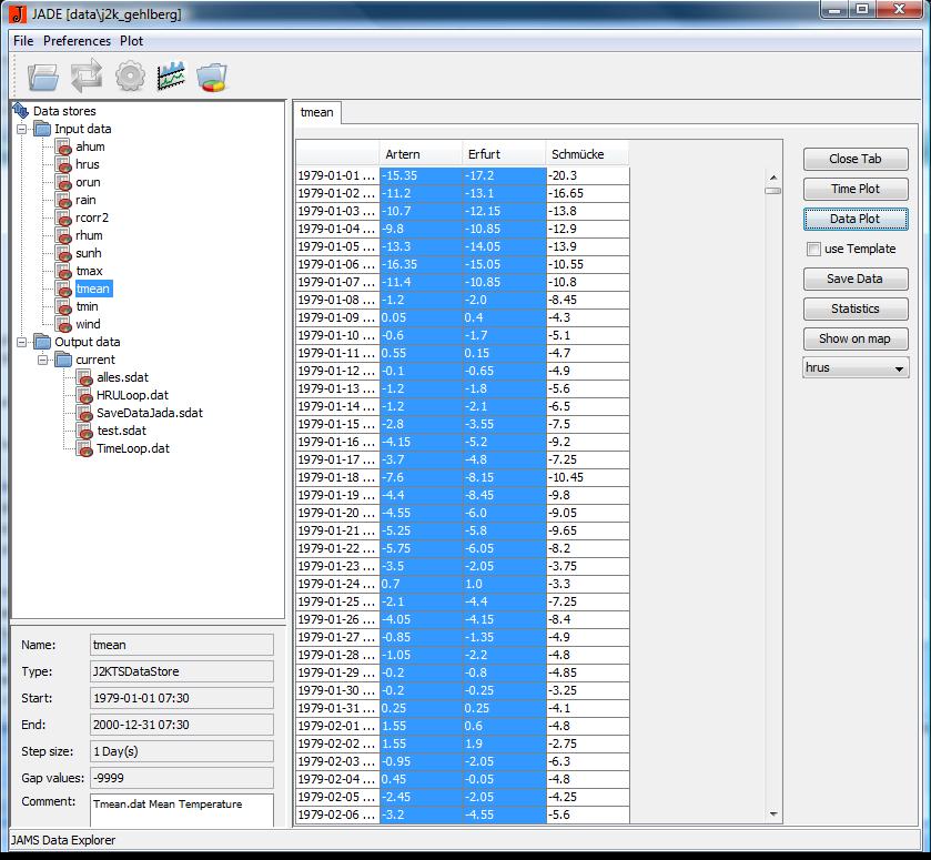
In order to evaluate the input data which were used for the modeling please select a data set from the input folder by double-clicking on the file. The selected data will be displayed in the box on the right side.
This example shows data of the tmean data set (mean temperature).
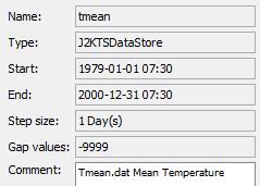
The box at the bottom left contains information on the data set:
- Name of the data series
- Data type
- Starting point of the time scale
- End point of the time scales
- Data density (step size between two data sets)
- Default value, in case no data are available
In the right hand box the selected data are displayed. The example shows that the measurement data were used at three different stations (Artern, Erfurt, Schmücke).
The key on the right hand side contains the following functions:
- Close Tab - closes data set.
- Time Plot - displays the selected data set (of at least one station) in a diagram. The point in time corresponds to the x-axis.
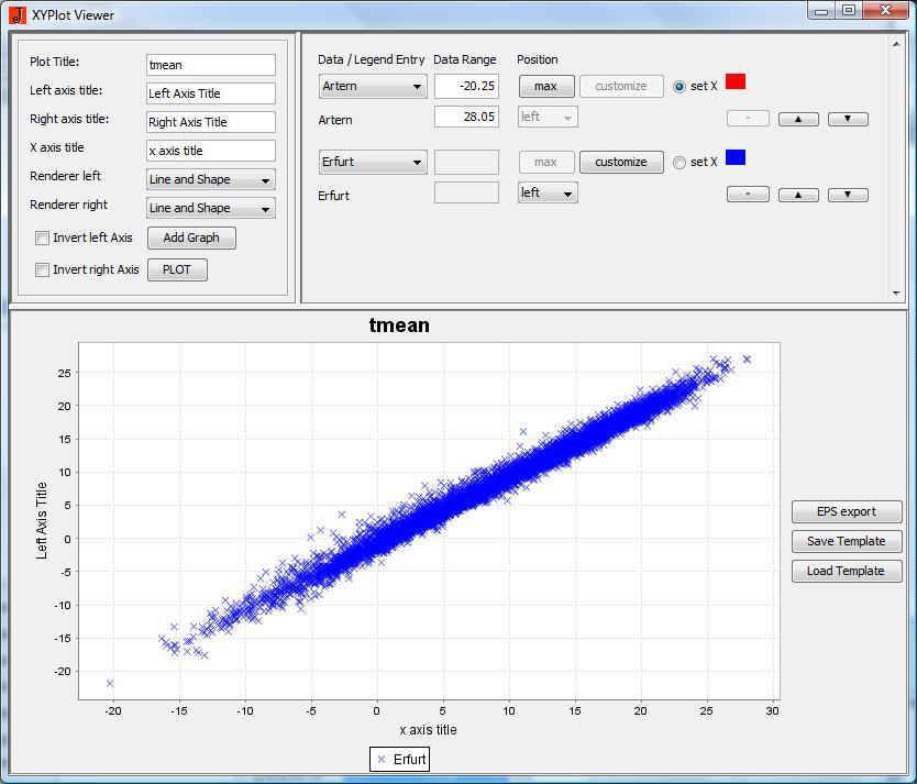
- Data Plot - displays comparison of data sets of at least two different stations in a diagram.
- Save Data - the selected data set can be saved.
- Statistics - statistical analysis of the selected data set(s).
Example
The following example shows the selection of the data set Erfurt by clicking on the button Erfurt.
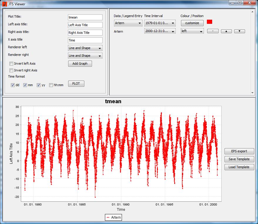
By clicking on the button Time Plot the time scale for the measuring station Erfurt is displayed in a diagram.
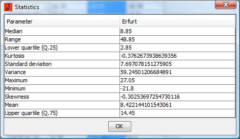
By clicking on the button Statistics the time scale for the measuring station Erfurt is evaluated.
Analysis of Output Data after the Modeling
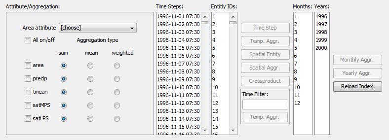
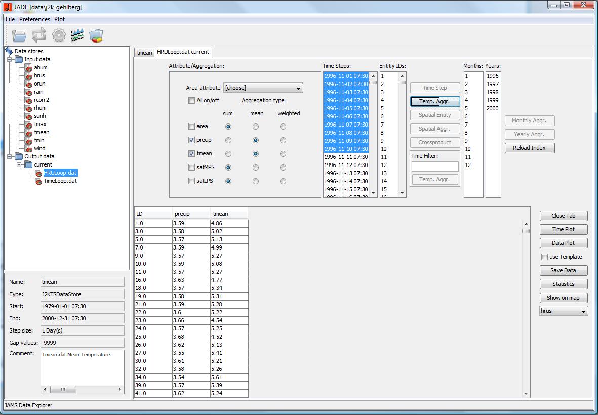
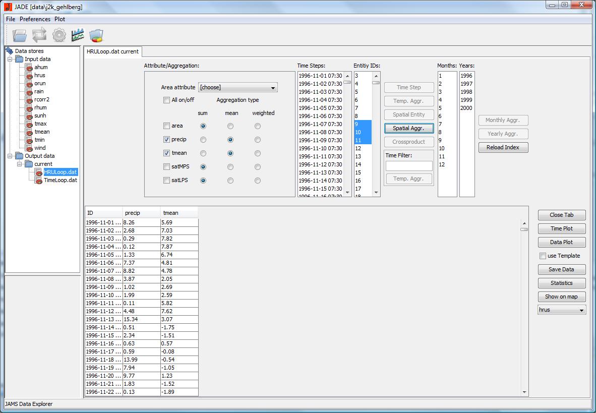
The data which are generated during the modeling can be analysed and visualized by using JADE. By double-clicking on the relevant data set, e.g. HRU Loop, a window opens for selecting data which are supposed to be analyzed in more detail. It is shown at the top right corner of the program surface which is shown in the following image.
In the first window attributes for the analysis can be chosen. In this case, those are area (of the HRU), precip (precipitation), tmean (mean temperature), satMPS (saturated middle pore storage) and satLPS (saturated large pore storage). For the aggregation type (1) the sum, (2) the mean and (3) the analysis according to the size of the HRU can be calculated/carried out. In the boxes Time Steps or Entity IDs time steps and elements (HRUs) can be selected. By using the shortcut Strg+A all time steps or elements can be selected altogether.
The following buttons are available:
- Time Step - Lists the selected data of the chosen time step for all HRUs.
- Temp. Aggr. - Lists the selected data of the chosen time step in an aggregated manner for all HRUs.
- Spatial Entity - Lists the selected data of the chosen HRUs for all time steps.
- Spatial Aggr. - Lists the selected data of the chosen HRUs in an aggregated manner for all time steps.
- Crossproduct - Lists the selected data of the chosen time step(s) for the chosen HRU(s).
- Time Filter - The time filter offers the possibility of listing aggregated data for particular months or years.
To show the aggregated value for November 1996, you would enter 1996-11-% in the time filter and then confirm with button Temp. Aggr..
In the boxes Month and Years it is possible to analyze particular months or years.
- Monthly Aggr. - Lists the selected data of the chosen month in an aggregated manner for all HRUs.
- Time Step - Lists the selected data of the chosen year in an aggregated manner for all HRUs.
- Reload Indes - Resets the selection.
Example
In this example, the data for the selected attributes of precipiation (precip) and mean temperature (tmean) from 1st November 1996 until 10th November 2006 are laoded in an aggregated manner. The aggregation type is the mean (Aggregation type = mean), i.e. the mean of the values (01.11.1996, 02.11.1996,...,10.11.1996) is calculated. Close Tab, Time Plot, Data Plot, Save Data, Statistcs and Show on map have been explained unter the item Analysis of Input Data for the Modeling.
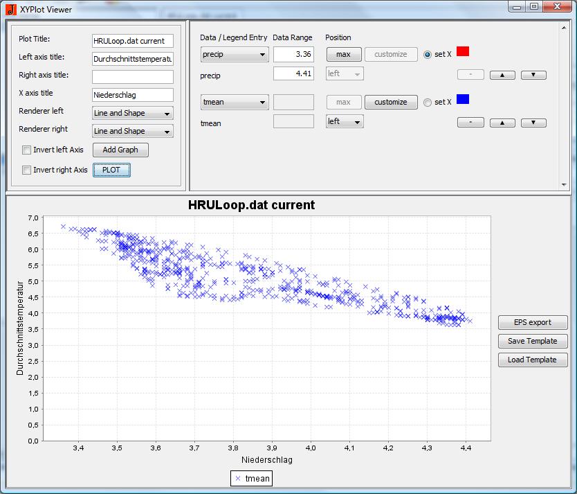
By clicking on the button Data Plot the following window is generated, where mean temperature (of the day) is related to precipitation.
Overview of Implemented Models
This tutorial is concerned with the hydrological modelling system J2000. The hydrological modelling system J2000g was developed as a simplified model and the modelling system J2000-S additionally takes into account the water and nitrogen budget. Therefore, the models can be seen as a simplification and an extension of the J2000. The modeling systems are introduced below.
J2000
The hydrological modeling system J2000 allows a physically-based modeling of the water supply of big catchment areas. Alongside the simulation of hydrological processes, which influence the runoff generation and its concentration on the upper meso and macro level, it contains routines which can most certainly be used to regionalize measured climate and precipitation data selectively available. In addition, the calculation of actual stand evaporation is directly integrated into the model which allows an area-specific calculation of the evaporation according to different land use classes. Since the model is supposed to be suitable for modeling large catchment areas with a size of several 1000km2, it is ensured that the modeling can be done with data available on a national scale. The simulation of different hydrological processes is carried out in closed program modules which are to a great extent independent of each other. This allows changing, substituting or adding single modules without having to structure the model once again from the start.
J2000-S
The water and mass transfer model J2000-S allows the simulation of the water and nitrogen budget of mesoscale catchments. The model is an extension of the model J2000 and therefore shares most components to describe the hydrological cycle. The description of the nitrogen budget contains additional components, naming soil temperature, soil nitrogen budget, land use management, plant growth and groundwater nitrogen budget. Additional modules were adjusted for requirements of the nitrogen budget.
J2000g
The model J2000g was developed as a simplified hydrological model to calculate temporally aggregated hydrological target figures distributed over time. Hydrological processes are calculated and displayed one-dimensionally for a random amount of points in space. Those modeling points allow an equal implementation of different distribution concepts (Response Units, grid cells, partial catchment areas) without any further model adjustment. The temporal discretization of the modeling can take place in daily steps or monthly steps. During the modeling the following processes are calculated for each time step: regionalization of climate data to the respective model units, calculation of global and net radiation as input for the calculation of evaporation, calculation of land-cover-specific potential evaporation according to Pernmam-Monteith, snow accumulation and snowmelt, soil water budget, groundwater recharge, retardation of runoff (translation and retention).
Preparation of Input Data
Application of the Implemented Grass-HRU Toolkit
Please see GRASS-HRU.
Sensitivity Analysis and Parameter Optimization
In order to apply hydrological models successfully it is necessary to define model parameters accurately. A direct measurement of the parameters is mostly not possible, too expensive or there is no clear physical relation. For those reasons the parameters are adjusted in a trial and error process in so far that the simulated factors (e.g. runoff) correspond best to the values measured. This task can be time-consuming and difficult if the corresponding model is complex or has a large number of parameters. Therefore it makes sense to automatize the optimization process with a software tool for the optimization of model parameters and sensitivity analysis which is available. Its functionality is described in detail in the Tutorial Calibration and Sensitivity Analysis.
Exercises for the Tutorial Basic Users
Exercise 1/JADE
Task
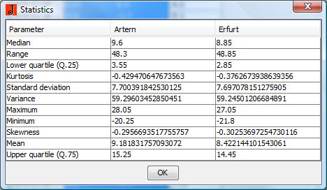
Please analyze the data set wind (wind) which was used for modeling the catchment area of the Wild Gera (water gage: Gehlberg). Select data sets for the measurement stations of Artern and Erfurt and have the data displayed in a diagram to compare them. Compare median, maximum and mimnimum of the time scales.
Solution
(1) Click on the tmean folder of the input data.
(2) Select the data sets of Artern and Erfurt (hold Ctrl and click on the data set). Now they should be highlighted in BLUE.
(3) By clicking on the button Data Plot the time scales for the measuring stations Artern and Erfurt will be compared in a diagram.
(4) By clicking on the button Statistics the selected time scales will be statistically analyzed. Thus, values for median, maximum and minimum can be read.
Exercise 2/ JADE
Task
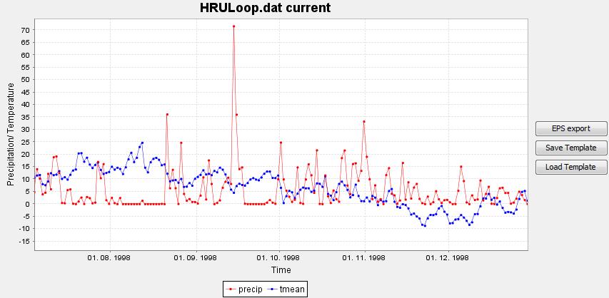
Analyze the precipitation and mean daily temperature of the model unit 9,10,11 (Entity IDs 9,10,11) of the modeling with the system J2000 in the catchment area of the Wild Gera with the water gage Gehlberg. In order to do so, calculate the mean of the three model units.
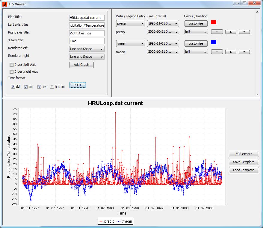
Show the data in a diagram. Modify the names of the axes according to the attributes which are displayed.
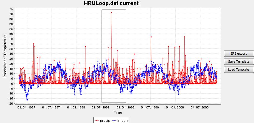
Zoom in the time period of 1st July 1998 until 31st Dec. 1998 and show it in a diagram.
Solution
(1) Click on attributes precip and tmean.
(2) Select mean as aggregation type.
(3) Select the three model units 9,10,11. (Tip: By holding the key Ctrl you can select several model units.)
(4) Click the button Spatial Aggr..
The following window should appear:
(5) Select the data sets ID,precip and tmean. (CTRL + click on the data set) It should be highlighted in BLUE now.
(6) Click on the button Time Plot to display the selected data. (The time axis will be automatically chosend to be the x-axis!)
(7) Select the period from 1st July 1998 until 31st Dec. 1998 by clicking on it.
(8) The required time period will be automatically displayed.
