From ILMS-Wiki
(Difference between revisions)
|
|
| Line 42: |
Line 42: |
| | The export delivers a tab stop splitted tet file. The header contains most important metadata information: Name of the RBIS (e.g. Okavango Basin Information System), Date of download, user name, dataset title, station name, coordinates and spatial reference system, elevation, time series ID, metadata ID and column description. The example shows a complete dataset without gaps. If data had or have data gaps you will further get the information of applied interpolation methods, date of interpolation and a declaration of completeness in the txt file. | | The export delivers a tab stop splitted tet file. The header contains most important metadata information: Name of the RBIS (e.g. Okavango Basin Information System), Date of download, user name, dataset title, station name, coordinates and spatial reference system, elevation, time series ID, metadata ID and column description. The example shows a complete dataset without gaps. If data had or have data gaps you will further get the information of applied interpolation methods, date of interpolation and a declaration of completeness in the txt file. |
| | | | |
| − | == Gap filling toolbox ==
| |
| | | | |
| − | Identified data gaps can be filled either by the internal rule based gap filling toolbox or externally.
| |
| − |
| |
| − | === Internal interpolation methods===
| |
| − |
| |
| − | RBIS includes different internal interpolation methods. The methods are explained in the section "Internal Interpolation Method Set". You can chose between following internal interpolation methods:
| |
| − |
| |
| − | * '''''inverse distance weighting'''''
| |
| − |
| |
| − | Inverse distance weighted methods are based on the assumption that the interpolating surface should be influenced most by the nearby points and less by the more distant points. The interpolating surface is a weighted average of the scatter points and the weight assigned to each scatter point diminishes as the distance from the interpolation point to the scatter point increases.
| |
| − |
| |
| − | Inverse distance weighting (IDW) uses the maximum given number of stations. If this number is not available the number is reduced to the given minimum number of stations.
| |
| − |
| |
| − | '''[1] IDW (5-3)''' Inverse distance weighting (IDW) (max 5 stations - min 3 stations are used)
| |
| − |
| |
| − | '''[1a] IDW & elevation correction (5-3)''' Inverse distance weighting (IDW) with elevation correction (max 5 stations - min 3 stations are used). Elevation correction is done by adjusting the values of the used stations to the elevation of the source station. These corrected values are used for IDW. If IDW with elevation correction is not possible only IDW is used instead. The default exponent is 2 otherwise it can be changed by the value of the parameter field.
| |
| − |
| |
| − |
| |
| − | * '''''linear regression'''''
| |
| − |
| |
| − | Linear regression is an approach to modeling the relationship between a scalar dependent variable y and one or more explanatory variables denoted X. The case of one explanatory variable is called simple regression. More than one explanatory variable is multiple regression.
| |
| − |
| |
| − | '''[2] linear regression''' with the values of the station with the best r² is used.
| |
| − |
| |
| − | '''[2a] linear regression (0.7''') Linear regression with the values of the station with the best r² in a radius of 10 stations is used if r² is at least 0.7 or greater.
| |
| − |
| |
| − | '''[2b] linear regression (0.7/30km)''' Linear regression with the values of the station with the best r² in a radius of 10 stations which is at least 0.7 or greater is used. The maximum distance of this station is 30km.
| |
| − |
| |
| − |
| |
| − | * '''''linear interpolation'''''
| |
| − |
| |
| − | Linear interpolation is a method of curve fitting. If two known points are given (value before and after gap), the linear interpolant is the straight line between these points. The default exponent is 2, otherwise it can be changed by the value of the parameter field.
| |
| − |
| |
| − | '''[3] linear interpolation'''
| |
| − |
| |
| − | '''[3a] linear int/regr. (l3/0.7)''' Linear interpolation is used if gap length is not more than 3. Gaps greater 3 are closed by linear regression with the values of the station with the best r² in a radius of 10 stations is used if r² is at least 0.7 or greater.
| |
| − |
| |
| − |
| |
| − | * '''''nearest neighbor'''''
| |
| − |
| |
| − | Nearest-neighbor interpolation (also known as proximal interpolation or, in some contexts, point sampling) is a simple method of multivariate interpolation in one or more dimensions.
| |
| − | Interpolation is the problem of approximating the value of a function for a non-given point in some space when given the value of that function in points around (neighboring) that point. The nearest neighbor algorithm selects the value of the nearest point and does not consider the values of neighboring points at all, yielding a piecewise-constant interpolant.
| |
| − |
| |
| − | '''[4] nearest neighbour'''
| |
| − |
| |
| − |
| |
| − | ''screen method selection''
| |
| − |
| |
| − | [[File:OBIS_Timeseries_InternalInterpolation.png|600px|]]
| |
| − |
| |
| − | === Define rules for interpolation methods===
| |
| − |
| |
| − | The user selects one method or can chose a combination of interpolation methods. In addition the user has the possibility to define rules for the application of the method by clicking on "''Internal Interpolation Method Set"''. A description of the method is given here. With support of selected rules the interpolation method can be adapted. Here values can be set for the parameters: length of data gap until the method shall be applied, maximum and minimum station number, coefficient of determination r2 and maximum distance. To set a maximum length of data gap is especially recommended for the linear interpolation method as this method is not suitable for larger data gaps. If you want to change the default setting, click on the button "Edit". Default values have been set, e.g. maximum number of stations is 5, minimum nuber is 3 and the minimum coefficient for determination was set to 0.7.
| |
| − |
| |
| − | The section "Internal Limit values" offers a table containing the value range of all parameters, e.g. humidity: minimum value is 0, maximum value is 100.
| |
| − |
| |
| − | Interpolation cannot be conducted in case that no matching time series were found or no matching method was found.
| |
| − |
| |
| − | ''screen internal interpolation method set''
| |
| − |
| |
| − | [[File:OBIS_internal_interpolation_method_set.png|1000px|]]
| |
| − |
| |
| − | ===External interpolation===
| |
| − |
| |
| − | The section "External Interpolation" offers the possibility to conduct an interpolation out of the OBIS and upload the file into OBIS.
| |
| − | If you use an external method you need to chose the method in the selection menue or describe a new method. The import function takes only those values which lie within a previously described data gap, even if the timeseries is longer. The values within the data gap were treated by OBIS like interpolated values. The gap interval can only be filled completely or not. If only one value in the timeseries is missing, it will not be used to close the gap.
| |
| − |
| |
| − | Further you need to specify the upload file. You can chose ''add'' to complement the timeseries or ''new'' to add new data after you have previously deleted already exitsing data. This feature allows to close still existing gaps without losing former interpolation results.
| |
| − |
| |
| − | [[File:OBIS_External_Interpolation.png|400px|]]
| |
| | | | |
| | [[Using_the_Okavango_Basin_Information_System_(OBIS)|[Back to tutorial main page]]] | | [[Using_the_Okavango_Basin_Information_System_(OBIS)|[Back to tutorial main page]]] |
Revision as of 08:31, 13 March 2013
The section time series data is one of the core features of OBIS. OBIS allows the management, visualization and download of time series data.
[Back to tutorial main page]
View list of available datasets
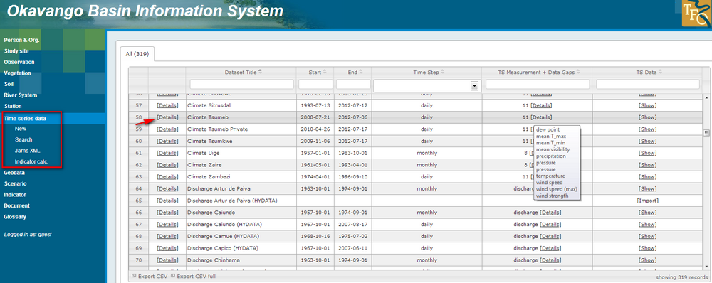
The section "Time series data" gives first an overview of all datasets. The measured data are directly linked to the stations, where they have been measured. The link "Export CSV" on the bottom of the table gives the possibility to download a list of all records you see in the overview table. The menu on the left side offers different features like the import of data, Jams XML and Indicator calculation. The tutorial will introduce these functions in the section Adding and modifying data - Time series data. At this stage you will learn how to browse for data, search data and view the time series data.
On the screen most important information are listed:
- Dataset title consists of measured parameter and station name, e.g. "Climate Benguela"
- Start of time series (yy-mm-dd)
- End of time series (yy-mm-dd)
- Time step, e.g. daily, monthly
- TS Measurement + Data Gaps, e.g. precipitation, discharge
- TS Data contains the link to access the data [show]
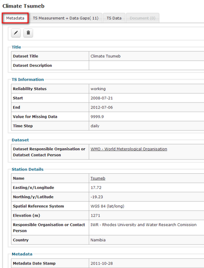
Metadata
For showing all information connected to a dataset you need to click on "details" in the row of a dataset you are interested in, e.g. the example "Climate Luanda".
First metadata are listed. They are grouped in Title, Time series information, Dataset and Station details.
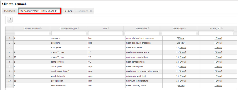
If you click in the register "TS Measurements + Data Gaps" time series connected to the station Luanda were displayed. For the example Luanda eight time series are available. There exists one time series for each parameter, e.g. temperature, precipitation, humidity and others. Further you ahve the possibility to show nearby stations. This feature is explained in the section Find nearby stations.
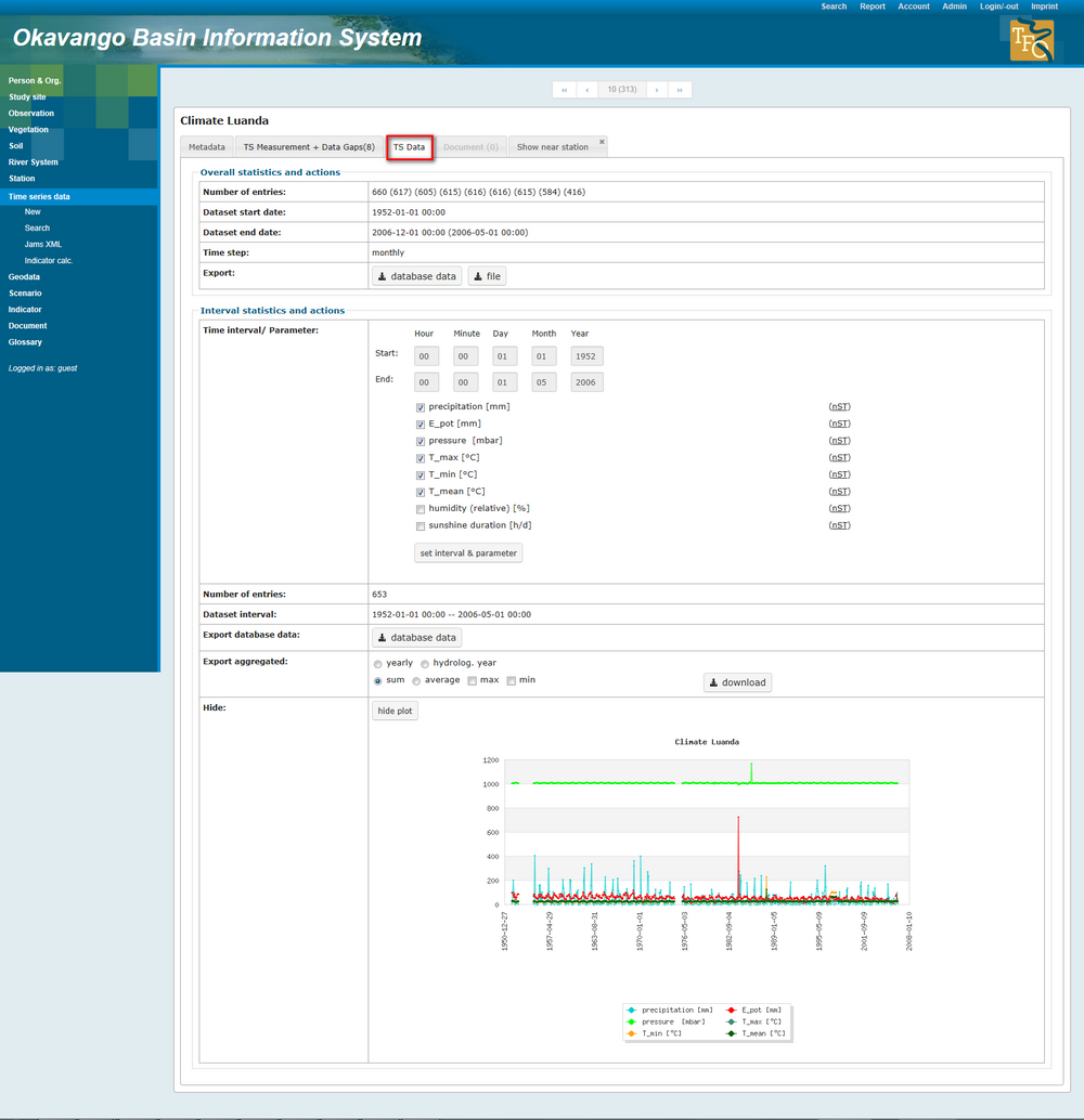
View and download time series data
The section "overall statistics and actions" lists the number of entries in total and the number of entries for each parameter in brackets. You get an overview of the completeness of the time series or number of gaps. Start and end date of the time series is shown. For the export of data you have two possibilities: If you are interested in the entire dataset, use the download link "database data" and you get a txt-file containing all data and metadata. The example "climate Luanda" file opened in an editor (see figure below), shows you station information and time series information, lists the parameters in their correct order and gives you the monthly data. Using this download link you get the data as they are stored in the database (no default values, no date gaps).
Using the download link "file" the original file will be exported as it has been uploaded to the database.
In the section "Interval statistics and actions" you have the possibility to view the time series data in a plot. You can set a time interval and parameters of interest. Therefore enter the time interval in the entry fields, activate the checkboxes of the parameters of interest and confirm the selection by clicking "set interval & parameter". By clicking on the link "show plot" a graph appears visualizing time series data for the timeframe and parameters selected before. By clicking on the link "database data" you get the time series for this respective timeframe and parameters. You can also chose the function "Export aggregated" for download. This feature allows to export e.g. yearly data, average data, max or min values or sum. Tick the checkboxes of the required output and click on "download".
Visualization of a txt-file in PSPad (download via the link "database data")
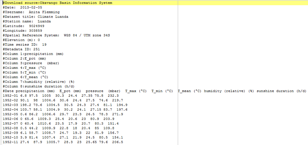
The export delivers a tab stop splitted tet file. The header contains most important metadata information: Name of the RBIS (e.g. Okavango Basin Information System), Date of download, user name, dataset title, station name, coordinates and spatial reference system, elevation, time series ID, metadata ID and column description. The example shows a complete dataset without gaps. If data had or have data gaps you will further get the information of applied interpolation methods, date of interpolation and a declaration of completeness in the txt file.
[Back to tutorial main page]


