JAMSSCS
Contents |
JAMSSCS
JAMSSCS is a program for the calculation of design discharges for small homogeneous catchment areas. For this purpose, JAMSSCS implements the unit-hydrograph method of the U.S. Soil Conservation Service (SCS) together with the Curve Number (CN) method for the effective rainfall. The program enables the estimation of the runoff in consideration of an approach of a specific design depth of precipitation for small homogeneous catchment areas. The calculations are carried out as far as possible according to the German DVWK rules 112/1982 and 113/1984 and have been adjusted and changed at some points.
JAMSSCS uses the Jena Adapatable Modelling System (JAMS) and is completely written in JAVA. Therefore, it is usable independently from the operating system on different computer configurations.
Note: The decimal separator is the . (period) and not the , (comma) for the data input.
Installation and Quick Start
thumb|Figure 1: JAMSSCS main window The installation in MS-Windows is carried out via the execution of the installation file "JAMSSCS_setup.exe". This file contains all necessary files for the execution. Additionally, a sample dataset is contained which can be used for a test and as template for the generation of new datasets. This manual uses this dataset. The installation file copies the necessary files and registers JAMSSCS in the start menu. A desktop icon can also be generated.
To tart JAMSSCS, double click on "JAMSSCS.exe". Hereupon, the main window of JAMSSCS appears (JAMS-launcher). The main window contains three tabulators (main group, Kostra-precipitation, individual event), which offer different functions. For the execution of the test dataset only the working directory needs to be set up. The complete path to the JAMSSCS installation directory has to be given here.
With the button [RUN] the model is started. thumb|Figure 2: runtime window of JAMSSCS
A new window with three tabulators appears. The first one [JAMSProgress] represents general information on the current model run as text. Should an error or problem arise while executing, an error message might appear in this view. The second tabulator [design discharge] shows the hydrograph of the design discharge in m³/s. The third tabulator [design volume] shows the cumulated volume in million m³. You can zoom into the graphics by left mouse click and pushing of the window. By right mouse click into the graphic a menu opens which allows a certain adjustment, e.g. changing the diagram title, labeling of the axes, background color, frame color, etc. Furthermore, the diagram can be saved as PNG graphic via this menu. The hydrograph can be switched on or off with the help of the checkbox on the right side.
JAMSSCS Input Data
Information that is provided for JAMSSCS always follows a strict format. For tables it is defined as follows:
- Rows that are introduced by # are comment rows which are not processed by the program. Comment rows are only allowed at the beginning of the table. There is no limitation of their number.
- The tabulator is always the column separator
- The order of the columns must always follow the order in the sample tables.
- The first row which is not introduced by # has to contain the row labeling. This labeling should always correspond to the labeling of the tables x and y. The program differentiates between upper and lower case.
- The following rows contain the actual information (separated by the tabulator).
JAMSSCS needs information about the research area and at least the design depth of precipitation. Additionally, a KOSTRA-precipitation file can be read in which contains precipitation heights for different durations and return periods. This file can be read out in XML-format from the KOSTRA-DWD software and can then be processed directly in JAMSSCS.
The necessary area information consists of a description of the hydrological homogeneous areas (HRUs – Hydrological Response Units) that exist in the area given in tables (HRU-table). The output criterion for the generation is the land use and soil type. The calculation of the desired CN-value is carried out on the basis of the reference table (CN table). In the installation there are examples given for both tables which can be adjusted, changed or added. Newly generated input tables for the area description can be given in the main window.
CN Table
The JAMSSCS CN table contains "Curve-Numbers" for different land use-soil-combinations and can be found in the installation directory as “cnNumbers.par”. The Curve-Number describes the part of precipitation that is runoff-effective. It can be interpreted as relative part. The actual calculation of the effective rainfall is described further down with the help of the curve-number.
Tabelle 1: Die CN table of JAMSSCS
| #CN-Numbers | |||||
| LID | soil use | A | B | C | D |
| 1 | settlement (neatly builded) | 80 | 80 | 80 | 80 |
| 2 | settlement (loosely builded) | 38 | 73 | 89 | 98 |
| 3 | farmland | 64 | 76 | 84 | 88 |
| 5 | deciduous forest | 36 | 60 | 73 | 79 |
| 6 | coniferous forest | 25 | 55 | 70 | 77 |
| 7 | bush, scattered fruit | 45 | 66 | 77 | 83 |
| 9 | grassland | 30 | 58 | 71 | 78 |
| 10 | open areas | 80 | 80 | 80 | 80 |
| 11 | water areas | 100 | 100 | 100 | 100 |
After the comment in the first row, the table contains the column labeling which do not need to be formulated exactly as it is shown here but can also be labeled differently. Note: The order of the columns must be kept in this order. The columns contain:
- LID: A numeric key number for a land cover or land use type, e.g. 3 for farmland (column 1).
- soil use: A description of the referring land cover or land use type in text form (column 2).
- A, B, C, D: SCS soil types that are described further down (columns 3, 4, 5, and 6).
Then, the entries for the single land cover categories in LID form, description, Curve Number for soil type A, B, C and D follow in the rows. The table can be expanded user-defined via entering new datasets if required. At this, the soil types are defined as follows:
- A: Soils with high infiltration capacity also after heavy pre-moistening, e.g. deep sand or gravel soils.
- B: Soils with middle infiltration capacity. Deep to moderate deep soils with moderate fine or rough texture, e.g. middle deep sand soils, loess, sandy clay.
- C: Soils with low infiltration capacity. Soils with fine to moderate fine texture or water damming layer, e.g. flat sand soils, sandy clay.
- D: Soils with very low infiltration capacity. Clay soils, very flat soils above nearly impermeable material, soils with always high groundwater level.
HRU table
The HRU table contains information about the research area and is structured as follows: (see table 2)
Table 2: HRU table with area information
| #hrus.par | |||
| "ID" | "AREA" | "LID" | "SID" |
| 1 | 0.011 | 3 | B |
| 2 | 1.39 | 4 | B |
| 3 | 0.156 | 7 | B |
| 4 | 0.014 | 8 | B |
| 5 | 0.3 | 11 | B |
The first row without introducing comment symbol (#) contains the labeling for the intern given variables.
The JAMSSCS-component, which this table reads, was generated in a way so exported GIS tables can be read in without further processing. For this reason the labeling must be given exactly as shown above. The permissible labeling are ID, SID, LID, AREA. The names do not need to be given in inverted commas. The order as well as upper and lower case are not important in this table. In addition to the tabulator, the comma (,) can be used as column separator, here.
The first column contains a clear numeric identification number for each hydrological unit; the second column contains the area (in m²), the third one contains the ID (LID) of the dominant land use of the table according to table 1. The fourth column contains the dominant soil type (A-D) – also according to table 1. For the processing of other areas the HRU table always needs to be generated. This can be carried out directly from a GIS. (Tools for automatized derivation in ArcView are described below.)
Further Input Data
thumb|Figure 3: The different precipitation allocations of JAMSSCSthumb|Figure 4: Sum functions of the different precipitation allocations of JAMSSCS The other necessary input data is given directly in the JAMSSCS main window (Figure 1). It is:
- Receiving stream length: The maximum length of the main receiving stream from the source to the runoff in kilometers.
- Deepest, highest point: The topographic height in meters of the deepest point (runoff) and of the highest point (source) of the main receiving stream.
- N-allocation form: Determines the temporal allocation of precipitation. Valid information is: B = block rainfall, rainfall M = in the middle of the event, A = at the beginning of the event and E = at the end of the event .
- Model runtime: Calculation time for the modeling in hours.
- Time step length: Length of a specific calculation time step in seconds.
For the precipitation allocation form the referring temporal allocations are implemented in JAMSSCS and follow the DVWK 113/1984 as far as possible.
Calculation of Individual Events
Individual precipitation events can be simulated with the help of the tabulator individual events. The necessary parameters can be adjusted here. These are:
- Precipitation duration: the temporal duration of precipitation in minutes
- Design depth of precipitation: the amount of fallen precipitation in open land which is reduced to effective rainfall in the model run
- Individual-Q-output: file name for an output file that is to be generated in which the calculated values can be saved. It is a simple ASCII-file which can be further processed with text editors as well as table calculations. The file name has to be given in consideration to the working directory. The file contains the runoff in m³/s for each time step as well as the temporally cumulated runoff volume in million m³.
- Decimal places: the number of decimal places for the values in the output file.
- Runoff-plot: the graphic output of hydrographs can be switched on or off here
The following fields serve the configuration of the model output. These are:
- Legend: labeling of the legend which is additionally complemented automatically by the precipitation height
- Line color: labeling for the color of the hydrograph. Valid labeling are for example "blue", "red", "green", "black" etc.
- X,Y-axes labeling: axes labeling (can also be changed later)
- Volume-plot: generates a graphic presentation of the temporally cumulated runoff volume in million m³.
Calculation with KOSTRA-Precipitation
thumb|Figure 5: Input tabulator for KOSTRA simulations with variable durations and return periods as well as extreme precipitation (PEN) thumb|Figure 6: KOSTRA simulation with fixed duration and variable return period thumb|Abb. 7: Figure 7: KOSTRA simulation with variable duration and fixed return period The product KOSTRA-DWD contains the storm rainfall heights for Germany in dependence of the duration and return period in the area of the durations D between 5 minutes and 72 hours as well as in the area of the yearly return periods between T = 0.5 a (according to the yearly exceedence frequency of n = 2x per year in the mean) and T = 100 a (in the mean all 100 years only once received or exceeded according to n = 0.01).
KOSTRA-DWD allows the export as XML-file which can be read directly from JAMSSCS. Such a file contains all values of a KOSTRA-DWD grid cell.
The calculations are carried out with the precipitation allocation form given in the tabulator main group. Further necessary settings are provided in the tabulator KOSTRA precipitation in JAMSSCS. These are:
- Kostra on: Switches KOSTRA calculations on or off
- Kostra-runoff-plot: Switches the graphic output of the hydrograph for KOSTRA calculations on or off
- Kostra-volume-plot: Switches the graphic output of the cumulated volume for KOSTRA calculations on or off
- Kostra-input-file: the exported XML-file from KOSTRA-DWD. The complete path name has to be given here, e.g. E:\Projekte\JAMSscnMethod\KOSTRA-DWD-Tabelle-S48-Z56 Jena.xml.
- Return period: either one of the valid KOSTRA return periods (0.5, 1, 2, 5, 10, 20, 50, 100) or each other return period which must be bigger than 100 years, though. The referring precipitations are calculated according to the PEN-method in this case. If a return period of more than 100 years is chosen in the field, the checkbox “PEN-precipitation on:” must be selected.
- Kostra-detail: a file name for the detail text output of a KOSTRA simulation. The file name is completed intern via the working directory. This file contains runoff data for each time step and for each combination of a KOSTRA simulation. The output format is a text file separated by tabulator.
- Kostra-summary: a compressed form of the results of a KOSTRA simulation which contains the maximum peak discharge and the volume of each calculated KOSTRA simulation
- Decimal places: the number of decimal places for the values in the output file
- Variable precipitation return period: If the checkbox is activated, the calculation with the precipitation duration, given in the tabulator individual event, and all return periods shown above is carried out. The valid precipitation durations are: 5, 10, 15, 20, 30, 45, 60, 90, 120, 180, 240, 360, 540, 720, 1080, 1440, 2880, 4320 minutes.
- Variable precipitation duration: If the checkbox is activated (and the one above is deactivated), the calculation for the return period given above and all precipitation durations given above is carried out.
- PEN-precipitation on: with the help of this checkbox the calculation of precipitation with very high return periods, which go beyond the 100 years return interval of the KOSTRA-values, is switched on or off. (The calculation of the PEN-precipitations is described further down.)
- PEN return periods: a list of return periods for which the PEN-calculation shall be carried out. The values of the list have to be separated by semicolon (;).
Interne Berechnungen - SCS Theorie, PEN-Niederschläge
Die interne Berechnung der Einheitsganglinie beruht auf der Berechnung des Effektivniederschlags in Abhängigkeit des CN-Wertes des Einzugsgebiets und einer linearen Speicherkaskade (Nash-Kaskade) mit zwei Speichern, mit unterschiedlichen Auslaufkoeffizienten (k1,2) sowie der variablen Verteilung des Niederschlages auf die beiden Speicher. Die erste Speicher repräsentiert dabei den schnellen Direktabfluss, der zweite den verzögerten Basisabfluss.
CN-Wert Berechnung
Für das Gebiet wird ein flächengewichteter mittlerer CN-Wert, basierend auf den Einträgen der HRU-Tabelle und der CN-Tabelle berechnet. Die Berechnung erfolgt nach:
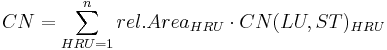
wobei rel.Area der relative Flächenanteil der HRU und CN(LU, ST) der der HRU entsprechende Eintrag in der CN-Tabelle ist.
Der Effektivniederschlag
Der Effektivniederschlag (hNe) beschreibt die abflusswirksame Menge des Gesamtniederschlags. Die Berechnung erfolgt nach folgender Potenzfunktion:
![h_{Ne} = \frac{\left[ (h_N / 25.4) - (200/CN) + 2 \right]^2}{(h_N / 25.4) + (800 / CN) - 8} \cdot 25.4](/ilmswiki/uploads/math/8/2/d/82d7134d815cb6e36678c73f7a44d724.png)
wobei: hN der Bemessungsniederschlag (in mm) und CN der CN-Wert nach Gleichung 1 ist. Die Untergrenze für den Bemessungsniederschlag (UGN), ab der ein Effektivniederschlag > 0 entsteht, ergibt sich durch Nullsetzen von hNe nach:
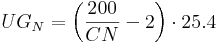
Bei einem Bemessungsniederschlag kleiner oder gleich der Untergrenze (UGN) ergibt sich damit ein Effektivniederschlag von 0 mm.
Aufteilung des Effektivniederschlags
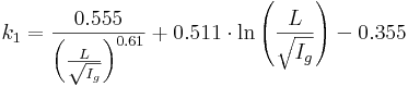
Der nach den oben dargestellten Gleichungen bestimmte Effektivniederschlag wird auf die beiden Speicher der Speicherkaskade durch Berechnung der Koeffizienten β1,2 aufgeteilt. β1 berechnet sich aus der Vorfluterlänge (L) und dem Vorfluter Gefälle (Ig = (HP – TP) / L) nach:
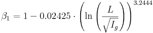 für
für 
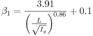 für
für 
Der Koeffizient β2 ergibt sich als 1 – β1. Durch diese Aufteilung erhält der erste Speicher (Direktabflussanteil) der Kaskade bei steilem Gebiet verhältnismäßig mehr Niederschlag und bei flacherem Gebiet verhältnismäßig weniger.
Die lineare Speicherkaskade
Die Berechnung der Einheitsganglinie erfolgt durch eine lineare Speicherkaskade mit zwei Speichern, die unterschiedliche Retentionskoeffizienten (k1,2) besitzen. Diese berechnen sich nach:
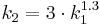
Für jeden der beiden Speicher wird dann eine Einheitsganglinie (Unit-Hydrograph) basierend auf den k-Werten nach folgender Gleichung berechnet:
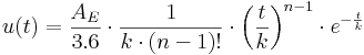
mit:
| t | der Zeitschritt in Sekunden |
| AE | die Größe des Einzugsgebiets in km² |
| n | die Anzahl der Speicher (hier immer 2) |
| k | der Retentionskoeffizient nach den oben angeführten Gleichungen |
Der Gesamtabfluss des Gebietes ergibt sich dann aus der Summe der beiden Abflusskomponenten.
Praxisrelevante Extremwerte des Niederschlags (PEN)
Die Abschätzung von Niederschlägen mit Jährlichkeiten oder Wiederkehrintervallen, die seltener als die 100 Jahre der KOSTRA-Daten sind, erfolgt nach modifiziertem PEN-Verfahren (Gewässerkundlicher Landesdienst Thüringen: Anforderungen an Hydrologische Gutachten, Fassung vom 31. Mai 2005). Mit diesem Verfahren werden die Niederschläge für beliebige seltene Wiederkehrintervalle ausgehend von den KOSTRA-Daten für jede KOSTRA-Dauerstufe extrapoliert.
Die Berechnung für einen Niederschlag P mit einem Wiederkehrintervall T und einer beliebigen Dauerstufe erfolgt nach:
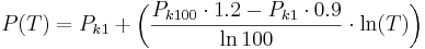 ,
,
wobei Pk1 der KOSTRA-Niederschlag mit Wiederkehrintervall 1 Jahr und Pk100 der KOSTRA-Niederschlag mit Wiederkehrintervall 100 Jahre der entsprechenden Dauerstufe ist.
HRU Parameter Bestimmung in ArcView
Mit dem GIS ArcView kann die Parametertabelle relativ einfach erzeugt werden. Die notwendigen Daten und Arbeitsschritte werden im Folgenden erläutert.
Notwendige Datenflächen
Für die Bearbeitung müssen folgende Datenflächen verfügbar sein:
- Bodenkarte mit CN-Kodierung (A-D) - liegt für gesamt Thüringen vor (Die Eingangkarte muss in der Attributtabelle ein Feld mit Namen "SID" enthalten, in der die CN-Kodierung (A-D) abgelegt ist!)
- Landnutzung mit entsprechender Kodierung - liegt für gesamt Thüringen vor (Die Eingangkarte muss in der Attributtabelle ein Feld mit Namen "LID" enthalten, in der die eindeutige numerische Kodierung für die Landnutzungseinheiten abgelegt ist!)
- Eine Shapedatei der Einzugsgebietsgrenze
- Eine Shapedatei des Hauptvorfluters (optional)
- Ein digitales Geländemodell (optional)
Alle Datenflächen müssen in einem einheitlichen Bezugssystem (z.B. Gauss-Krüger) vorliegen.
Voraussetzungen in ArcView
thumb|Abb. 8: Auswahl der "Geoprocessing" ErweiterungEs müssen folgende Erweiterungen (Extensions) installiert und aktiviert sein:
- Geoprocessing
- Spatial Analyst (nur notwendig, wenn Höhenmodell verwendet wird)
- JAMSSCS Erweiterung (jamsscs.avx)
Die Erweiterung jamsscs.avx (die oben heruntergeladen werden kann) muss in das Erweiterungsverzeichnis (EXT32) von ArcView kopiert werden. Im allgemeinen befindet sich dies unter: C:\ESRI\AV_GIS30\ARCVIEW\EXT32.
Die Installation der JAMSSCS Erweiterung fügt in ArcView ein neues Menü (JAMSSCS) hinzu, das sichtbar ist, wenn ein View aktiv ist. Dieses Menü enthält drei Einträge, die weiter unten ausführlicher beschrieben werden.
Ob die Erweiterungen installiert und aktiviert sind, lässt sich über den Menupunkt: Datei --> Erweiterungen überprüfen.
Zuschneiden der Eingangsdaten
thumb|Abb. 9: Dialog zum Zuschneiden der EingangsdatenZur Erzeugung der Flächeninformation müssen zunächst die Bodenkarte mit CN-Kodierung und die Landnutzungskarte für das relevante Einzugsgebiet zugeschnitten werden. Dies erfolgt mit dem "GeoProcessingWizard", den drei Eingangskarten (Bodenkarte, Landnutzungskarte, Einzugsgebietsgrenze), die in ArcView geöffnet sein müssen und folgenden Arbeitsschritten:
- Start des "GeoProcessingWizard" aus dem Menu JAMSSCS --> GeoProcessing...
- Auswahl des Unterpunktes "Ausschneiden (Clip)" im erscheinenden Dialog und betätigen des [Weiter] Knopfes
- Auswahl von Bodenkarte oder Landnutzungskarte in der oberen ListBox ("Auszuschneidendes Eingabethema auswählen:") und die Einzugsgebietsgrenze in der zweiten ListBox ("Polygon Überlagerungsthema auswählen:"). Bei beiden Eingaben muss die CheckBox "Nur ausgewählte Objekte verwenden" abgewählt sein.
- Optional kann ein Ausgabedateiname in der dritten ListBox ("Ausgabedatei angeben") angegeben werden.
- Mit dem Knopf [Fertigstellen] wird der Prozess gestartet.
Wenn die oben angeführten Arbeitsschritte für die beiden Eingangskarten durchgeführt wurden, stehen nun zugeschnittene Versionen der Landnutzungs- und Bodenkarte für die weitere Bearbeitung zur Verfügung.
Überlagern der Eingangsdaten
thumb|Abb. 10: Dialog zum Überlagern der Eingangsdaten Für die Überlagerung müssen die zugeschnittenen Karten der Landnutzung und der CN-kodierten Bodenkarte vorliegen. Die Überlagerung erfolgt mit dem "GeoProcessingWizard" der mit dem Menupunkt JAMSSCS --> GeoProcessing... gestartet wird. Dann müssen folgende Eingaben gemacht werden.
- Auswahl von "Themen verschneiden (Intersect)" dann Knopf [Weiter]
- Auswahl der ausgeschnittenen Landnutzung in der ersten ListBox
- Auswahl der ausgeschnittenen CN-kodierten Bodenkarte in der zweiten ListBox
- Optional kann ein Dateinamen für die Ausgabedatei (z.B. "hrus.shp") angegeben werden.
Mit dem Knopf [Fertigstellen] wird der Prozess gestartet. Als Ergebnis entsteht eine Karte, die die Kombination aus Landnutzung und CN-kodierten Bodentypen enthält.thumb|Abb. 11: Eingangsinformation, Überlagerung und Attributtabelle
Aktualisieren der Attributtabelle
Für den Einsatz in JAMSSCS muss die Attributtabelle des entstandenen HRU-Themas aktualisiert und erweitert werden. Im einzelnen:
- Hinzufügen einer eindeutigen numerischen Identifikationsnummer (ID) für jedes Polygon
- Entfernen überflüssiger Attribute
- Berechnung und Hinzufügen der Fläche in m² für jedes Polygon
Hierfür muss zunächst das HRU-Thema im View ausgewählt sein. Dann wird über den Menüpunkt "JAMSSCS --> Tabelle aktualisieren..." die Attributtabelle mit der notwendigen Information erweitert.
Exportieren der Attributtabelle
Die erweiterte Attributtabelle ist schließlich noch zu exportieren, um später mit JAMSSCS verarbeitet werden zu können. Hierzu muss das HRU-Thema im View aktiv sein. Der Export erfolgt dann mit dem Menüpunkt "JAMSSCS-->Tabelle exportieren...". Es wird noch ein Dateiname abgefragt und dann exportiert.
Literatur
DVWK-Regeln zur Wasserwirtschaft, H. 112/1982: Arbeitsanleitung zur Anwendung von Niederschlags-Abfluss-Modellen in kleinen Einzugsgebieten; verantw. Herausg. Dt. Verb. für Wasserwirtschaft u. Kulturbau e.V. (DVWK). Bearb. vom DVWK-Fachausschuss "Niederschlag-Abfluss-Modelle" - Hamburg, Berlin: Parey; Teil I: Analyse; DK 556.161.072 Niederschlag-Abfluss-Modelle, DK 556.51.028 Kleineinzugsgebiete. - 1982.
DVWK-Regeln zur Wasserwirtschaft, H. 113/1984: Arbeitsanleitung zur Anwendung von Niederschlags-Abfluss-Modellen in kleinen Einzugsgebieten; verantw. Herausg. Dt. Verb. für Wasserwirtschaft u. Kulturbau e.V. (DVWK). Bearb. vom DVWK-Fachausschuss "Niederschlag-Abfluss-Modelle" - Hamburg, Berlin: Parey; Teil 2: Synthese; DK 556.161.072 Niederschlag-Abfluss-Modelle, DK 556.51.028 Kleineinzugsgebiete. - 1984.
Bearbeitung und Kontakt
| Dr. Peter Krause | Dr. Claudia Liese |
| Lehrstuhl Geoinformatik | Referat 51 - Gewässerökologie, Hydrologie, Wasserbau |
| Institut für Geographie | Abteilung 5 - Wasser, Boden, Altlasten, Wismut |
| Friedrich-Schiller-Universität Jena | Thüringer Landesanstalt für Umwelt und Geologie |
| Tel. 03641-948864 | Tel. 03641-684518 |
| email: p.krause@uni-jena.de | email: c.liese@tlugjena.thueringen.de |