Hydrological Model J2000g
Abstract
The Model J2000g was developed as a simplified hydrological model to calculate temporally aggregated, spatially allocated hydrological target sizes. The representation and calculation of the hydrological processes is carried out one-dimensionally for an arbitrary number of points in the space. These model points enable the use of different distribution concepts (Response Units, grid cells, catchment areas) without further model adjustments.
The temporal discretization of the modeling can be carried out in daily or monthly steps. During the modeling the following processes are calculated for each time step: regionalization of punctual existing climate data to the referring model units, calculation of global and net radiation as access for the evaporation calculation, calculation of the land-cover-specific potential evaporation according to Penman-Monteith, snow accumulation and snowmelt, soil water budget, groundwater recharge, retardation in runoff (translation and retention). The individual processes are described in more detail below.
Distribution and Attribute Tables
The model J2000g is not bound to any specific distribution concept because the processes are calculated on the basis of points in the space that are independent of each other (1D-model concept). These points can represent different space units, e.g. single station positions, polygons, grid cells, catchment areas or subcatchments but also rather administrative units such as field unit or administrative districts. In the following text the term “model unit” is used for these points.
Model Unit Attribute Table
Each model unit needs to be described with specific attributes for the modeling. These are:

- ID - a clear numeric ID
- X - the easting of the centre (centroid) as Gauss-Krüger coordinate
- Y - the northing of the centre (centroid) as Gauss-Krüger coordinate
- area - the area of the model unit in m²
- elevation - the mean elevation of the model unit in m above N.N.
- slope - the mean slope of the model unit in degree
- aspect - the aspect of the model unit in degree from North clockwise
- soilID - a clear numeric ID for the soil type (serves as allocation to the soil attribute table)
- landuseID - a clear numeric ID for the land use/land cover type (serves as allocation to the land use table)
- hgeoID - a clear numeric ID for the hydrological unit of the model unit (serves as allocation to the hydrogeology table)
The model unit attribute table contains the attribute names in the first row. These must not be changed because they are used as variable name for the attribute generation during the model parameterization. The second row contains the minimal possible value of the referring attribute, whereas the third one contains the maximum possible value. In the fourth row the physical unit of the attribute needs to be entered. Then, as many rows as needed are given that contain the attribute values of the single model units. The table needs to be completed by a comment row which starts with the comment symbol (#). The tab (\t) has to be used to separate the rows.
Soil Attribute Table

The soil attribute table contains soil-physical characteristics for each soil unit that occurs in the area. In the current model version only the usable field capacity for each decimeter is needed. On the basis of the field capacity the maximum storage capacity of the soil water storage is calculated in dependence of the effective root depth of the vegetation on the model unit during the model parameterization.
The format of the soil attribute table is very similar to the model units attribute table. The table can be started with an arbitrary number of comment rows that need to be started with the comment symbol (#). In the first interpreted row the attribute names need to be given. The spelling is very important here. The following attributes need to be included:
- SID - clear numeric ID with which the connection to the model unit table is generated
- depth - depth of the soil in cm
- fc_sum - entire usable field capacity of the soil in mm
- fc_1 bis fc_n - usable field capacity for each decimeter in mm/dm
To complete the table, a comment row must be given (introduced with #). The tab (\t) has to be used to separate the rows.
Land Use Attribute Table

The land use attribute table contains vegetation parameters that are nearly exclusively needed for the evaporation calculation according to Penman-Monteith. In the table the following attributes need to be given for each land use unit and land cover unit that occurs in the area:
- LID - a clear numeric ID with which the connection to the model unit table is generated.
- description - a description as text
- albedo - albedo [0 ... 1]
- RSC0_1 bis RSC0_12 - the stomatal resistances for good water availability for the months January (RSC0_1) to December (RSC0_12) in s/m
- LAI_d1 bis LAI_d4 - the area leaf index in m²/m² for the Julian Days 110 (d1), 150 (d2), 250 (d3) and 280 (d4) for a terrain height of 400 m above N.N.
- effHeight_d1 bis effHeight_d4 - effective vegetation height in meter for the Julian Days 110 (d1), 150 (d2), 250 (d3) und 280 (d4) for a terrain height of 400 m above N.N.
- rootDepth - the effective root depth in dm
To complete the table, a comment row must be given (introduced with #). The tab (\t) has to be used to separate the rows.
Hydrogeology Attribute Table

In the hydrogeology attribute table the maximum possible ground water recharge rates per time unit are set up for each hydrogeologic unit. It only contains the following two attributes:
- GID - a clear numeric ID with which the connection to the model unit table is generated.
- mxPerc - the maximum possible percolation rate (ground water recharge rate) per time interval in mm per time unit
To complete the table, a comment row must be given (introduced with #). The tab (\t) has to be used to separate the rows.
Input Data - Model Driver

For the model run climate time series of an arbitrary number of climate and precipitation stations are needed. The time series have to be preprocessed in the referring formatted data files. The files have the following format:
Rows 1 to 13 contain meta information about the data. They are arranged in blocks which are started with descriptions which in turn are started with the AT-symbol (@). Multiple entries per row are separated via the tab (\t).
- @dataSetAttribs (attribute of the dataset)
- missingDataVal - value that marks missing data
- dataStart - start date of the dataset (DD.MM.JJJJ HH:MM)
- dataEnd - end date of the dataset (DD.MM.JJJJ HH:MM)
- tres - termporal resolution (days "d", months "m")
- @statAttribVal (attributes of the climate stations)
- name - the names of the climate stations
- ID - a numeric, clear ID
- elevation - the elevation of the station in m above N.N.
- x - easting as Gauss-Krüger-coordinate
- y - northing as Gauss-Krüger-coordinate
- dataColumn - describes the column in which the data for the referring station can be found
In the following rows the actual data for each time step is listed – starting with:
- @dataVal
The format is Date, Time followed by Data that is separated by the tab.
Installation and Start
Model Initialization
Regionalization
The regionalization module is used for the transfer of punctual values to the model units. The procedure was taken from the hydrological Model J2000 without any changes and is arranged in the following steps:
- Calculation of a linear regression between the station values and the station heights for each time step. Thereby, the coefficient of determination (r2) and the slope of the regression line (bH) is calculated.
- Definition of the n gaging stations which are nearest to the particular model unit. The number n which needs to be given during the parameterization is dependent on the density of the station net as well as on the position of the individual stations.
- Via an Inverse-Distance-Weighted Method (IDW) the weightings of the n stations are defined dependently on their distances for each model unit. Via the IDW-method the horizontal variability of the station data is taken into account according to its spatial position.
- Calculation of the data value for each model unit with the weightings from point 3 and an optional elevation correction for the consideration of the vertical variability. (The elevation correction is only carried out when the coefficient of determination –calculated under point 1 – goes beyond the threshold of 0.7.)
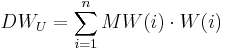
The calculation of the data value for each model unit (DWU) without elevation correction is carried out with the weightings (W(i)) and the values (MW(i)) of each n gaging station according to:
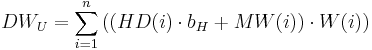
For the calculation with elevation correction the elevation difference (HD(i)) between the gaging station and the model unit as well as the slope of the regression line (bH) are taken into account. Thus, the data value for the model unit (DWU) is calculated according to:
Precipitation Correction
Precipitation values partly show a clear systematic error in measurement which is caused instrument-determined or due to the selection of the instrument position. This error in measurement has two causes: (1) the moistening error and evaporation error, which each depends on the type of the instrument and (2) the wind error which emerges due to the drifting of the precipitations. Both errors in measurement are strongly dependent on the type (rain or snow) of the precipitation amount.
For the correction of both errors a correction method according to Richter (1995) is used which is applied in the same way in the Model J2000. The procedure for the evaporation correction differs with regard to the temporal resolution of the precipitation data.
Monthly Precipitation Correction
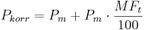
The corrected precipitation (Pkorr) is calculated for monthly time steps on the basis of the decrease of the measured precipitation (Pm) and the percental monthly error in measurement (MFt) (see adjacent table):
Daily Precipitation Correction
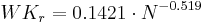
For the daily precipitation correction the two error terms are calculated explicitly. For this purpose, correction functions were derived on the basis of the tabled error values according to Richter (1995).
Moistening Loss and Evaporation Loss

For a continual error correction of the moistening loss and evaporation loss continual correction functions were adjusted to the tabled values by Richter (1995). They are shown in the adjacent figure. The correction functions were derived each separately for the winter half year (November till April) and summer half year (May till October). With these functions the moistening loss and evaporation loss is calculated in mm for precipitations <= 9 mm according to:


If the amount of precipitation is greater than 9 mm, a constant error of 0.47 mm in the summer half year and of 0.3 mm in the winter half year is assumed.
Wind Error

The calculation of the wind error of the precipitation measurement with the Hellman precipitation gauge is also carried out according to the tabled error values from Richter (1995) which was adjusted to the referring continual correction functions. For the correction it is differentiated whether the precipitation was rain or snow. The way of internal differentiation is described further below. The relative correction value is calculated as follows:
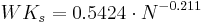 for snow
 for rain.
The corrected precipitation value (PK) is finally calculated on the basis of the value (PM), the relative correction value for the wind error (WKs, WKr) as well as the moistening loss and evaporation loss (BVSom, BVWin) as follows:

Radiation Calculation
For the evaporation calculation according to Penman-Monteith, the net radiation is needed as initial value and can be calculated on the basis of the global radiation. If the global radiation is not available, it can be defined approximately on the basis of the sunshine duration. For this purpose, a number of intermediate calculations are necessary. The following calculations act on the assumption of a daily modeling. When the model runs in monthly time steps, the calculations listed below are carried out on the 15th of each month. The resulting terms are then accumulated on the basis of the days per month.
Extraterrestrial Radiation

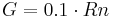
The extraterrestrial radiation (Ra) is the short-wave radiation energy flux of the sun at the upper boarder of the atmosphere. Ra is calculated for a specific place in dependence of its latitude (lat in radians), the declination of the sun (decl in radians), the solar constant (Gsc in MJ / m2min), the hour angle at sundown (ws in radians) and the inverse relative distance between earth and sun (dr in radians) according to:

The solar constant (Gsc in MJ / m2min) results from the Julian Date (jD [1... 365,366]) as follows:
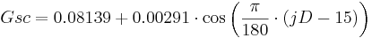 [MJ / m2min]
The relative distance between earth and sun (dr in radians) results from the Julian Date (jD [1... 365,366]) as follows:
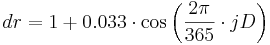 [rad.]
The declination of the sun (decl in radians) results from the Julian Date (jD [1... 365,366]) as follows:
 [rad.]
The hour angle at sundown (ws in radians) results from the latitude (lat in radians) and the declination (decl in radians) as follows:
 [rad.]
Global Radiation
The global radiation (Rg) is calculated on the basis of the extraterrestrial radiation (Ra in MJ/m²d) and the degree of cloudiness. At this, the degree of cloudiness is approximated on the basis of the relation of the measured sunshine duration (D in h/d) to the astronomic possible sunshine duration (S0 in h/d) with the help of the Angström formula. Thus, Rg is calculated as follows:
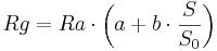 [MJ/m²d]
The coefficients a and b need to be estimated for the position. Often 0.25 is used for a and 0.50 is used for b.
The maximum astronomic possible sunshine duration (S0 in h) is calculated on the basis of the hour angle at sundown (ws in radians) as follows:
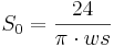 [h/d]
[h/d]
Net Radiation
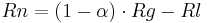
The net radiation (Rn in MJ/m²d) results from the single radiation components and provides the energy for the evaporation. The net radiation is calculated on the basis of the difference of the global radiation (Rg in MJ/m²d) and the effective long-wave radiation (Rl in MJ/m²d). The global radiation is reduced by the albedo (alpha) of the referring land cover.
The effective long-wave radiation (Rl in MJ/m²d) is calculated on the basis of the Bolzmann constant (Bk = 4.903E-9 MJ/K4m²d), the absolute air temperature (Tabs in K), the actual vapor pressure of the air (ea in kPa), the actual global radiation (Rg in MJ/m²d) and the maximum global radiation for unclouded sky (Rg0 in MJ/m²d):
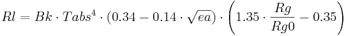 [MJ/m²d]
The actual vapor pressure of the air (ea in kPa) is calculated on the basis of the saturation vapor pressure (es in kPa) and the relative humidity (U in %) according to the following equation:
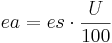 [kPa]
[kPa]
The saturation vapor pressure of the air (es in kPa) results from the air temperature (T in °C) according to:
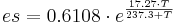 [kPa]
[kPa]
The maximum global radiation for uncovered sky (Rg0 in MJ/m²d) results from the extraterrestrial radiation (Ra in MJ/m²d) and the terrain height (h in m above N.N.) as follows:
 [MJ/m²d]
Evaporation Calculation
The calculation of the potential evaporation can be carried out according to Penman-Monteith or Haude. The advantage of the Penman-Monteith method is the higher physical basis. However, much more input data is needed. For the calculation according to Haude only air temperature and relative humidity are required.
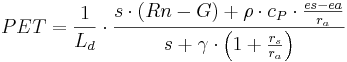
Potential Evaporation according to Penman-Monteith
The calculation of the Bestandesverdunstung according to Penman-Monteith (PET in mm/d) is calculated as follows:
 [mm/d]
with:
Ld : latent heat of evaporation [MJ/kg]
s : slope of the vapor pressure curve [kPa / K]
Rn : net radiation [MJ/m²d]
G : soil heat flux [MJ/m²d]
ρ : density of the air [kg/m³]
cP : specific heat capacity of the air (=1.031E-3 MJ/kg K]
es : saturation vapor pressure of the air [kPa]
ea : actual vapor pressure of the air [kPa]
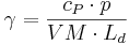
γ : psychrometer constant [kPa / K]
ra : aerodynamic resistance of the land cover [s/m]
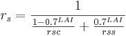
rs : surface resistance of the land cover [s/m]
The latent heat of evaporation (Ld in MJ/kg) results from the air temperature according to the following equation:
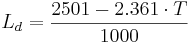 [MJ/kg]
The slope of the saturation vapor pressure curve (s in kPa/K) is calculated on the basis of the air temperature:
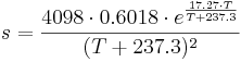 [kPa/K]
The soil heat flux (G in MJ/m²d) results from the net radiation (Rn in MJ/m²d):
 [MJ/m²d]
The density of the air (ρ in kg/m³) results from the air pressure (p in kPa) and the virtual temperature (vT in K):
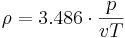 [kg/m³]
If the air pressure (p in kPa) is not available as value, it can be calculated approximately on the basis of the terrain height (h in m ü.NN) and the absolute air temperature (Tabs in K) according to the following equation:
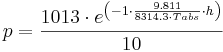 [kPa]
[kPa]
The virtual temperature (vT in K) results from the air pressure (p in kPa), the absolute air temperature (Tabs in K) and the actual vapor pressure of the air (ea in kPa):
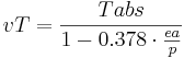 [K]
[K]
The psychrometer constant (γ in kPa / K) is calculated on the basis of the specific heat capacity of the air (=1.031E-3 MJ/kg K), the air pressure (p in kPa), the relation of the molecular weight of dry and humid air (VM = 0.622) and the latent heat of evaporation (Ld in MJ/kg):
The surface resistance of the land cover (rs in s/m) results from the leaf area index LAI, the stomatal resistance for the given point in time (rsc in s/m) and the surface resistance of an uncovered surface (rss = 150 s/m) as follows:
The aerodynamic roughness of the land cover (ra in s/m) results from the wind speed (v in m/s) and the effective vegetation height (eH in m)
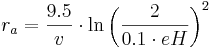 [s/m] for stands with eH < 10 m
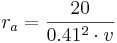 [s/m] for stands with eH >= 10 m
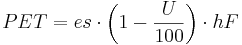
Potential Evaporation according to Haude
The potential evaporation according to Haude is calculated on the basis of the saturation deficit of the air and an empirical, dimensionless Haude-factor (hF). The saturation deficit results from the saturation vapor pressure (es in kPa) and the relative air humidity (U in %). The Haude-factor has to be defined for different vegetation types. The calculation of the potential evaporation (PET in mm) is carried out according to:
The saturation vapor pressure of the air (es in kPa) results from the air temperature (T in °C):
[kPa]
Snow Cover Calculation
The snow cover calculation is implemented as simple accumulation and snowmelt approach. The method decides on the basis of the air temperature whether water is saved as snow on a model unit or whether potentially existing snow melts and produces snowmelt runoff. For this purpose, two temperatures are calculated from the minimum temperature (Tmin), average temperature (Tavg) and maximum temperature (Tmax) of the referring time step:
The accumulation temperature as: 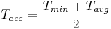 [°C] and
the snowmelt temperature as: 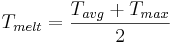 [°C]
[°C]
If the accumulation temperature (Tacc) lies on or below a threshold (Tbase) that needs to be given by the user, it is assumed that potentially occurring precipitation falls as snow. It is then saved on the model unit.
If the snowmelt temperature goes beyond the temperature threshold Tbase, the snowmelt is calculated with the help of a simple snowmelt factor (TMF). For this purpose, a potential snowmelt rate is calculated on the basis of the TMF (in mm/d K), the temperature threshold and the snowmelt temperature:
 [mm/d]
This potential snowmelt rate is then compared to the actual saved snow water equivalent which is then partly or fully melted. The resulting snowmelt water is passed on as input to the following module.
Soil Water Budget
The soil water budget module serves as allocator of the input (precipitation and snowmelt) to the output paths (evaporation, direct runoff, ground water recharge). The central element is the soil storage which is dimensioned via the usable field capacity of the rooted soil area. The maximum fill volume can be adjusted by a multiplicative user-controlled calibration parameter (FCA).
First, the input (precipitation and snowmelt) is allocated to the evaporation until the potential evaporation is reached. The surplus (inflow) is then allocated in direct runoff (SQ) and infiltration (INF), in dependence of the relative soil saturation (Θ) and a calibration parameter (DFB). The calculation is carried out as follows:
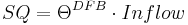 [mm/d]
 [mm/d]
The infiltration (INF) is allocated to the soil storage until it is completely saturated. If there is a surplus (excess water EW), it is allocated to the two paths interflow (SSQ) and ground water recharge (GWR) in dependence of the slope (α) and a calibration parameter (LVD). The calculation is carried out according to the following equation:
 [mm/d]
 [mm/d]
The ground water recharge is seen as source for the basis runoff (BQ) now.
Runoff Concentration and Retardation in Runoff
The runoff concentration and retardation in runoff is represented as simple function of the catchment area for the three runoff components (direct runoff, SQ, intermediate runoff SSQ and basis runoff BQ). For this purpose, the generation rates of the three components are accumulated area-weighted and are lead by their own linear cascade (Nash-cascade). For each of the three cascades the user has to determine the following two parameters: number of storages (n) and retention coefficient (k).