Hydrological Model J2000

From ILMS-Wiki

Revision as of 11:36, 11 November 2013 by Bjoern (Talk | contribs)

(diff) ← Older revision | Latest revision (diff) | Newer revision → (diff)

The hydrologic model system J2000 offers a physical-based modeling of the water balance of big catchment areas. In addition to the simulation of hydrologic processes, which influence the runoff and its concentration in the upper meso- and macro scale, the modeling system contains routines that help to regionalize the punctual available climate values and precipitation values quite safely. Furthermore, the calculation of the real evaporation, with which the calculation is carried out area-differentiated in consideration of the evaporation patterns of different land use classes, is integrated into the model. Since the model shall be suitable for the modeling of big catchment areas of more than 1000 km², it is ensured that the modeling can be carried out by means of the available base data on the national scale. The simulation of the different hydrologic processes is carried out in program modules that are completed and as far as possible independent of each other. This offers to edit, substitute or add individual modules without the necessity to structure the entire model anew. The modeled total runoff is built up on the sum of the individual runoff components that are separately calculated during the modeling. The modeling system differentiates between four runoff components according to their specific origin. The component with the highest temporal dynamics is the fast direct runoff (RD1). It consists of the runoff of sealed areas, of snow water, which drains within snow layers, and of surface runoff when saturation areas develop. The slow direct runoff component (RD2), which can be regarded as similar to the lateral hypodermic runoff within the soil zone, reacts insignificantly slower. Two further basis runoff components can be distinguished. On the one hand, there is the fast basis runoff component (RG1) which simulates the runoff from surface-near well permeable weathering zones. On the other hand, there is a slow basis runoff component (RG2) which results as runoff from joint aquifer or homogeneous loose rock aquifer. The allocation of the precipitation water to the individual runoff components is carried out in the model on the basis of area parameters which can be derived from the applied base data. In addition to the relief shape, specific soil parameters, like the hydraulic conductivity of individual soil horizons, have an important influence. The calculation of the runoff components’ different concentration times is carried out in consideration of the hydraulic characteristics of the storages in which the individual components drain. Additionally, variable influences like the preceding soil moisture of the area are considered while modeling.

1 GUI
2 Input files
- 2.1 Data
- 2.2 Parameters
3 Regionalization of Climate and Precipitation Data
- 3.1 General Processing
- 3.2 Specific Correction Method and Calculation Method for the Individual Datasets
4 Calculation of Evapotranspiration
5 Interception Module
6 Snow Module
7 Soil Water Module
8 Ground Water Module
9 Lateral Routing
10 Reach Routing

GUI

After starting JAMS, the main window opens which contains several tabulators:

Basic Settings

Workspace directory: Sets the working directory. It has to contain three more folders: Parameter (for all parameter files), Data (for all data files) and Output (for all output files).

Time interval: The time interval for the model run is selected.

Caching: The results of some compute-intensive processes can be temporarily stored in hard disk and reused for further model runs. Therefore the model run is slightly faster. Attention: This feature is not completely safe yet and should only be applied by experienced users.

Diagrams and Maps

Runoff plot: Activates the graphical display of the runoff modeled and measured during model run.

Soil moisture plot: Activates the graphical display of the relative soil moisture during model run.

Snow water equivalent: Activates the graphical display of the snow water equivalent during model run.

Map enable: Enables the output of a cartographic display of selected state variables.

Map attributes: A semicolon-separated list of state variables which are to be cartographically displayed.

Map3D enable: Enables a 3D output of a cartographic display of selected state variables.

Map3D attributes: A semicolon-separated list of state variables which are to be cartographically displayed (in 3D).

Initialising

Multiplier for field capacity : The maximum storage capacity of the middle pore storages (MPS) can be increased (value > 1) or decreased (value < 1).

Multiplier for air capacity: The maximum storage capacity of the large pore storages (LPS) can be increased (value > 1) or decreased (value < 1).

initRG1: relative filling of the upper groundwater storage at beginning of model run (1 filled to capacity, 0 empty).

initRG2: relative filling of the lower groundwater storage at beginning of model run (1 filled to capacity, 0 empty).

Regionalization

number of closest stations for regionalization: Number n of stations used to calculate the value of an HRU (n stations which are closest to the HRU are selected).

Power of IDW function for regionalization: Weighting factor used to exponentiate the distance of each station to the respective HRU.

elevation correction on/off: Activates the elevation correction of the data values.

r-sqrt threshold for elevation correction: Threshold value for the elevation correction of the data values. If the coefficient of determination of the regression relation between measured data of the stations and station elevations is smaller than this value, an elevation correction is not carried out.

Those settings (i.e. minimum temperature, maximum temperature, medium air temperature, precipitation, absolute air moisture, wind speed, sunshine duration) can be adjusted for every single input variable.

Radiation

flowRouteTA [h]: runtime of the outflow route

Interception

a_rain [mm]: Maximum storage capacity of the interception storage per m² leaf area for rain

a_snow [mm]: Maximum storage capacity of the interception storage per m² leaf area for snow

Snow

Component active: Activates the snow module.

baseTemp [°C]: Temperature limit value for snow precipitation.

t_factor [mm/°C]: Temperature factor for calculation of snowmelt runoff.

r_factor [mm/°C]: Rain factor for calculation of snowmelt runoff.

g_factor [mm]: Soil heat flux factor for calculation of snowmelt runoff.

snowCritDens [g/cm³]: critical snow density

ccf_factor [-]: factor for calculation of the cold content of snow cover

Soilwater

MaxDPS [mm]: maximum hollow reserve

PolRed [-]: polynomial reduction factor for reduction of potential evaporation with limited water supply.

LinRed [-]: linear reduction factor for reduction of potential evaporation with limited water supply.

(Note: PolRed and LinRed do not represent alternatives. Only one can be attributed a value, the other one has to be 0.)

MaxInfSummer [mm]: maximum infiltration during summer period

MaxInfWinter [mm]: maximum infiltration during winter period

MaxInfSnow [mm]: maximum infiltration with snow cover

ImpGT80 [-]: relative infiltration capacity of areas with a sealing degree of > 80%

ImpLT80 [-]: relative infiltration capacity of areas with a sealing degree of < 80%

DistMPSLPS [-]: calibration coefficient for distribution of infiltration on soil storages LPS and MPS

DiffMPSLPS [-]: calibration coefficient for the definition of the diffusion amount of the LPS storage in relation to MPS at the end of a time step

OutLPS [-]: calibration coefficient for definition of LPS outflow

LatVertLPS [-]: calibration coefficient for distribution of the LPS outflow on the lateral (interflow) and vertical (percolation) component

MaxPerc [mm]: maximum percolation rate

ConcRD1 [-]: retention coefficient for direct runoff

ConcRD2 [-]: retention coefficient for interflow

Groundwater

RG1RG2dist [-]: calibration coefficient for distribution of percolation water

RG1Fact [-]: factor for runoff dynamics of RG1

RG2Fact [-]: factor for runoff dynamics of RG2

CapRise [-]: factor for the setting of capillary rise

Routing in the Flow

flowRouteTA [h]: runtime of the outflow route

When all parameters are set, the modeling is initiated via the button [Run]. A window opens which contains different tabulators.

The tab [JAMSProgress] represents general information about the current model run in text form. If an error or problem occurs during the implementation, an error message possibly appears in this view. Furthermore, different efficiency criteria are given after the completion of the model run. These are:

e2 ... Nash-Sutcliff-efficiency with power 2 (classic form)

e1 ... modified Nash-Sutcliff-efficiency (differences are not squared but their absolute values are applied)

log_e2 ... modified Nash-Sutcliff-efficiency (the logarithm of the values are taken)

log_e1 ... modified Nash-Sutcliff-efficiency (the logarithm of the values are taken; differences are not squared but their absolute values are applied)

ioa2 ... index of agreement according to WILLMOT

ioa1 ... modified index of agreement according to WILLMOT (differences are not squared)

r² ... coefficient of determination

grad ... slope of the regression line

wr² ... coefficient of determination, weighted with the slope of the regression line

dsGrad ... double sum gradient

AVE ... absolute volume error

RSME ... root mean square error

pbias ... relative percentage volume error

The further tabs contain the plots and maps selected beforehand.

Input files

Input files are the temporal static parameters as well as temporal variable input data (climate values, precipitation values, runoff values). These are read in as ASCII-Files.

Generally, for all input files it is necessary that:

the separator is the tabulator
the decimal separator is the dot

Data

The modeling system J2000 expects the following data files for the model initialization:

name	description	unit
ahum.dat	absolute humidity	g/cm³
orun.dat	measured flow passage at the runoff	m³/s
rain.dat	measured amount of precipitation	mm
rhum.dat	relative humidity	%
sunh.dat	sunshine duration	h
tmax.dat	maximum temperature	°C
tmean.dat	mean air temperature	°C
tmin.dat	minimum temperature	°C
wind.dat	wind speed	m/s

Each data file has the following structure (demonstrated here for the example of rainfall):

line	description
#rain.dat rainfall
@dataValueAttribs
rain 0 9999 mm	name of the data series, smallest possible value, biggest possible value, unit
@dataSetAttribs
missingDataVal -9999	value to mark missing data values
dataStart 01.01.1979 7:30	date and time of the first data value
dataEnd 31.12.2000 7:30	date and time of the last data value
tres d	temporal resolution of the data (here: days)
@statAttribVal
name stat1 stat2	names of the gaging stations
ID 1574 1513	numeric name of the gaging stations (ID)
elevation 525 498	elevation station1, elevation station2
x 4402310 4422269	easting station1, easting station2
y 5620906 5616856	northing station1, northing station2
dataColumn 1 2	number of the particular column in the data part
@dataVal	beginning of data part
01.01.1979 07:30 0.8 0.1	date, time, value station1, value station2
...
31.12.2000 07:30 1.1 0	date, time, value station1, value station2
#end of rain.dat	end of data part

Parameters

J2000 expects the following parameter files for the model initialization:

landuse.par – land use
hgeo.par - hydrogeology
soils.par – soil types
reach.par – net of water course
hrus.par – parameter of the derived Hydrological Response Units (HRUs)

Generally, all parameter files have the following structure (demonstrated here for the example of the net of water course; see also the figure on the right):

Sample of a parameter file

line	description
1	#reach.par
2	name of variable
3	smallest possible value
4	biggest possible value
5	unit
6	beginning of data part
n	#end of reach.par -> marks the end of the parameter file (here: land use)

landuse.par

parameter	description
LID	land use ID
albedo	albedo in %
RSC0_1	minimum surface resistance for water-saturated soil in January
...
RSC0_12	minimum surface resistance for water-saturated soil in December
LAI_d1	leaf area index (LAI) at the beginning of the vegetation period
...
LAI_d4	leaf area index (LAI) at the end of the vegetation period
effHeight_d1	effective vegetation height at the beginning of the vegetation period
...
effHeight_d4	effective vegetation height at the end of the vegetation period
rootDepth	root depth
sealedGrade	sealed grade

hgeo.par

parameter	description
GID	hydrogeology ID
RG1_max	maximum storage capacity of the upper ground-water reservoir
RG2_max	maximum storage capacity of the lower ground-water reservoir
RG1_k	storage coefficient of the upper ground-water reservoir
RG2_k	storage coefficient of the lower ground-water reservoir

reach.par

parameter	description
ID	channel part ID
length	length
to-reach	ID of the underlying channel part
slope	slope
rough	roughness value according to MANNING
width	width

soils.par

parameter	description
SID	soil type ID
depth	thickness of soil
kf_min	minimum permeability coefficient
depth_min	depth of the horizon above the horizon with the smallest permeability coefficient
kf_max	maximum permeability coefficient
cap_rise	Boolean variable, that allows (1) or restricts (0) capillary ascension
aircap	air capacity
fc_sum	useable field capacity
fc_1 ...22	useable field capacity per decimeter of profile depth

hrus.par

Parameters of the given Hydrological Response Units (HRUs)

parameter	description
ID	HRU ID
x	easting of the centroid point
y	northing of the centroid point
elevation	mean elevation
area	area
type	drainage type: HRU drains in HRU (2), HRU drains in channel part (3)
to_poly	ID of the underlying HRU
to_reach	ID of the adjacent channel part
slope	slope
aspect	aspect
flowlength	flow length
soilID	ID soil class
landuseID	ID land use class
hgeoID	ID hydrogeologic class

Regionalization of Climate and Precipitation Data

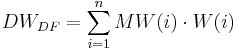
General Processing

1. Calculation of the linear regression between the daily station values and the elevation of the stations. . Thereby, the coefficient of determination (r²) and the slope of the regression line (b_H) of this relation is calculated. It is assumed that the value (MW) depends linearly on the terrain elevation (H); according to:

$MW = a_H + b_H \cdot H$

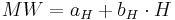
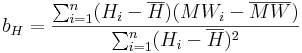
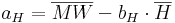
The unknown a_H and b_H are defined according to the Gaussian method of the smallest squares:

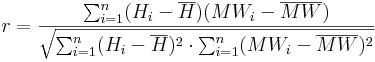
$b_H = \frac{\sum_{i=1}^{n} (H_i - \overline{H})(MW_i - \overline{MW})}{\sum_{i=1}^{n} (H_i - \overline{H})^2}$

$a_H = \overline{MW} - b_H \cdot \overline{H}$

The correlation coefficient of the regression is calculated according to the following equation:

$r = \frac{\sum_{i=1}^{n} (H_i - \overline{H})(MW_i - \overline{MW})}{\sqrt{\sum_{i=1}^{n} (H_i - \overline{H})^2 \cdot \sum_{i=1}^n (MW_i - \overline{MW})^2}}$

2. Definition of the n gaging stations which are nearest to the particular HRU.. The number n which needs to be entered during the parameterization is dependent on the density of the station network as well as on the position of the individual stations.

For each dataset the number of stations (n) that shall be considered for the regionalization needs to be determined in advance. Furthermore, a weighting factor (pIDW) needs to be given. The n-nearest stations are defined according to the following calculation rule with the help of the eastings and northings of all stations as well as the coordinates of the particular HRU. The first step is to calculate the distance (Dist(i)) of each station to the area of interest:

$Dist(i) = \sqrt{(RW_{stat(i)} - RW_{DF})^2 + (HW_{stat(i)} - HW_{DF})^2}$

with

RW ... easting of the station i...n, or the HRU (DF)

HW ... northing of the station i...n, or the HRU (DF)

The n stations with the smallest distance to the particular HRU are taken from the distances calculated according to the description above and are then used for further calculations. The distances of these stations are converted to weighted distances (wDist(i)) via potentialization with the weighting factor pIDW. With the help of this weighting factor the influence of nearby stations can be increased and the influence of more distanced stations can be decreased. Good results can be achieved with values of 2 or 3 for the pIDW.

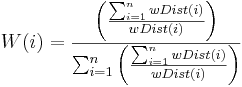
3. Via an Inverse-Distance-Weighted (IDW) the weightings of the n stations are defined dependently on their distances for each HRU. Via the IDW-method the horizontal variability of the station data is taken into account according to its spatial position. The calculation is carried out according to the following equation:

$W(i) = \frac{\left( \frac{\sum\nolimits^n_{i=1} wDist(i)}{wDist(i)} \right)}{\sum^n_{i=1}\left( \frac{\sum\nolimits^n_{i=1} wDist(i)}{wDist(i)} \right)}$

4. The calculation of the data value for each HRU with the weightings from point 3 and an optional elevation correction for the consideration of the vertical variability. The elevation correction is only carried out when the coefficient of determination (calculated under point 1) goes beyond the threshold entered by the user. The calculation without the optional elevation correction is carried out according to the following equation:

$DW_{DF} = \sum^n_{i=1} MW(i) \cdot W(i)$

For data values that possess an elevation effect, an elevation correction for the measured values is carried out additionally when the values have a tight regression relation (r² greater than the threshold entered by the user). The following equation is applied for the calculation:

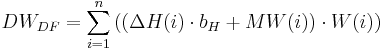
$DW_{DF} = \sum^n_{i=1} \left( ( \Delta H(i) \cdot b_H + MW(i)) \cdot W(i) \right)$

with ΔH(i) ... elevation difference between station i and the HRU

b_H ... slope of the regression line

Specific Correction Method and Calculation Method for the Individual Datasets

Precipitation

Correction of the Moistening Error and Evaporation Error

The correction of the moistening error and evaporation error is carried out according to researches with the help of Hellmann-rainfall gauges by RICHTER (1995). In order to offer a constant correction of the error (which results from the moistening and evaporation loss), logarithmic functions were approximated separately for the summer half year (May-October) and winter half year (November-April) to the discrete tabulated values in the modeling system 2000. If the precipitation height goes beyond the value of 9 mm the moistening error and evaporation error is set to a constant value.

The moistening error and evaporation error for precipitation heights ≤9.0 mm is calculated according to the following equates:

$BV_{Som}= 0.08 \cdot \ln{N} + 0.225 \; \; \; \mathrm{[mm]}$

$BV_{Win}= 0.05 \cdot \ln{N} + 0.13 \; \; \; \mathrm{[mm]}$

For precipitation heights >9.0 mm the moistening and evaporation error is:

$BV_{Som} = 0.47 \; \; \; \mathrm{[mm]}$

$BV_{Win} = 0.30 \; \; \; \mathrm{[mm]}$

Correction of the Wind Error

The quantification of the precipitation error that is to be expected is carried out according to the researches by RICHTER (1995) as function of the precipitation height and the position of the station. It is assumed that the relative wind error (KR_Wind) for rainfall as well as snowfall behaves inversely proportional to the precipitation heights (Pm). The calculation is carried out according to the following equations:

$KR_{Wind}= \begin{cases} 0.1349 \cdot P_m^{-0.494} & \mathrm{f\ddot{u}r} \; \; T_{mean} > T_{crit} \\ 0.5319 \cdot P_m^{-0.197} & \mathrm{f\ddot{u}r} \; \; T_{mean} \le T_{crit} \end{cases} \; \; \mathrm{[-]}$

The calculation of the precipitation heights corrected for evaporation error and wind error is then carried out according to the following equation:

$P_{korr} = P_m + P_m \cdot KR_{Wind} + BV_{Som}, BV_{Win} \, \, \, \mathrm{[mmd^{-1}]}$

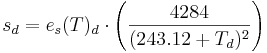
Temperature

The modeling system J2000 requires values of the day minimum temperature as well as the day maximum temperature. From these values the mean day temperature (T_mean) is calculated as mean average.

The regionalization of the punctual values T_min,T_max and T_mean is carried out according to the rule described above with optional elevation correction.

Wind Speed

The wind speed is not given as direct value from the DWD but as wind force observations (WS) in Beaufort. The conversion of the wind force into the wind speed at 2 m height (v₂) [in ms^-1] can be carried out according to the following equation:

$v_2 = 0.6 \cdot WS^{1.5} + 0.1 \; \; \; \mathrm{[ms^{-1}]}$

This conversion needs to be carried out externally, because J2000 expects the wind speed in m/s.

The conversion of the wind speed at 2 m height to other heights – as it is partly required during the evaporation calculation and the wind correction of the precipitation – is carried out during the modeling according to the following equation:

$v_z = \frac{v_z}{\left( \frac{4.2}{\ln z + 3.5}\right)} \; \; \; \mathrm{[ms^{-1}]}$

The interpolation of the punctual values to the area is carried out according to the method described above. The modeling system allows the inclusion of the optional elevation correction for the regionalization of the wind speed. However, this option should be handled with care, since the wind speed is very dependent on the station’s position.

Sunshine Duration

The daily sunshine duration (S) [in h], is provided as value by the DWD. The interpolation of the station values to the area is carried out according to the procedure described above – without additional calculations or elevation corrections.

Relative Humidity

The relative humidity (U) [in %] can be taken from the DWD as daily values. A direct regionalization of the values is not recommended since they depend on two parameters: the absolute moisture content and the maximum possible moisture content of the air for a particular temperature. Thus, in the J2000 modeling system’s regionalization module the absolute humidity (a) [in g cm^-3] is calculated from the relative humidity and the temperature at the station. It is then regionalized and afterwards the absolute humidity is converted to the relative humidity, again. For this purpose, several calculation steps are necessary which are shown below.

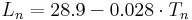
Calculation of the Saturation Vapor Pressure

The saturation vapor pressure (e_s(T)) [in hPa] is calculated according to the Magnus formula with the coefficients by SONNTAG (1994) for the air temperature (T) [in °C]:

$e_s(T) = 6.11 \cdot e^{\left( \frac{17.62 \cdot T}{243.12 + T} \right)} \; \; \; \mathrm{[hPa]}$

Calculation of the Maximum Humidity

The maximum humidity (A) is calculated against the saturation vapor pressure (e_s(T)) and the air temperature (T) according to:

$A(T) = e_s(T) \cdot \frac{216.7}{T + 273.15} \; \; \; \mathrm{[g cm^{-3}]}$

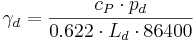
Calculation of the Absolute Humidity

The real water content of the air, the absolute humidity (a) [in gcm^-3], results from the maximum humidity (A)[in gcm^-3] and the relative humidity (U) [in %]:

$a = A \cdot \frac{U}{100} \; \; \; \mathrm{[g cm^{-3}]}$

The so calculated station values of the absolute humidity are then regionalized according to the procedure described above and are converted into relative humidity afterwards. The advantage of this rather complex regionalization method is that, in addition to its higher physical relation, the absolute humidity is more dependent on heights than the relative humidity. Thus, the elevation effect can be used for the regionalization according to the procedure described above. After the regionalization of the absolute humidity, the conversion into relative humidity can be carried out. However, instead of the temperature of the station, the previously regionalized average air temperature T_mean of the corresponding discrete sub-area is set.

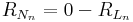
Calculation of Evapotranspiration

The calculation of the Bestandverdunstung is carried out in J2000 according to the Penman-Monteith equation in several steps in regard to numerous parameters. Since the calculation is very complex and time-consuming, it was sourced out into the preprocessing part of the modeling system. This outsourcing is possible because most of the parameters that are used for the calculation are derived from the input data and are thus seen as independent of the modeled dynamic of the water supply. The only parameter that is used in the calculation but can only be defined during the modeling is the current soil moisture. Its reducing influence is taken into account via appropriate reduction functions during the modeling. Two evaporation values are generated for each time interval (1 day) during the calculation of the evaporation. These values are a day value (index d) and a night value (index n). This distinction is necessary because the net radiation balance is very different at day or night. Furthermore, the evaporation behavior of the vegetation is different at day or night. In the night the plants’ stomata are closed, the surface resistance is unequally higher than at daytime. The calculation for the day and for the night is carried out according to the following equations, whereby the total value of the evaporation for the particular time step results as sum of these two values.

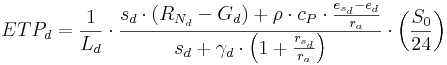
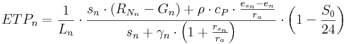
$ETP_d = \frac{1}{L_d} \cdot{ \frac{s_d \cdot {(R_{N_d} - G_d)}+ \rho \cdot{c_P} \cdot\frac{e_{s_d} - e_d}{r_a}}{s_d + \gamma _d \cdot{\left(1+ \frac{r_{s_d}}{r_a} \right)}}} \cdot{\left(\frac{S_0}{24} \right)}$

$ETP_n = \frac{1}{L_n} \cdot{ \frac{s_n \cdot {(R_{N_n} - G_n)}+ \rho \cdot{c_P} \cdot\frac{e_{s_n} - e_n}{r_a}}{s_n + \gamma _n \cdot{\left(1+ \frac{r_{s_n}}{r_a} \right)}}} \cdot{\left(1- \frac{S_0}{24} \right)}$

with:

L_d,n ... latent heat of evaporation [Wm^-2] per [mmd^-1]

s_d,n ... slope of the vapor pressure curve [hPaK^-1]

R_{N _d,n} ... net radiation [Wm^-2]

G_d,n ... soil heat flux [Wm^-2]

ρ ... density of the air [kgm^-3]

c_p ... specific heat capacity of the air for constant pressure [Jkg^-1K^-1]

e_{s_d,n} ... saturation vapor pressure [hPa]

e_d,n ... vapor pressure [hPa]

r_a ... aerodynamic resistance of the land cover [sm^-1]

γ _d,n ... psychrometer constant [hPaK^-1]

r_{s_d,n} ... surface resistance of the land cover [sm^-1]

S₀ ... astronomic possible sunshine duration [h]

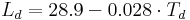
The air temperatures (T_d e T_n), which become necessary for the calculation of the net radiation balance, are derived from the values of the minimum temperature and maximum temperature as well as from the daily mean value:

$T_d = \frac{T_{max} + T_{mean}}{2} \, \, \, \mathrm{[C]}$

$T_n = \frac{T_{min} + T_{mean}}{2} \, \, \, \mathrm{[C]}$

The latent heat of evaporation (L) is calculated approximately according to:

$L_d = 28.9 - 0.028 \cdot{T_d}$

$\left[\frac{W}{m^2} \, \mbox{pro} \, \frac{\mathrm{mm}}{\mathrm{d}}\right]$

$L_n = 28.9 - 0.028 \cdot{T_n}$

The saturation vapor pressure (e_s(T)) of the air for the temperature (T) is calculated according to the Magnus formula with the coefficients by Sonntag:

$e_s (T)_d = 6.11 \cdot e^{\frac{17.62 \cdot{T_d}}{243.12 + T_d}} \, \, \, \mathrm{[hPa]}$

$e_s (T)_n = 6.11 \cdot e^{\frac{17.62 \cdot{T_n}}{243.12 + T_n}} \, \, \, \mathrm{[hPa]}$

The real vapor pressure (e) results from the saturation vapor pressure and the relative air humidity (U in [%]):

$e_d=e_s(T)_d \cdot \frac{U}{100} \, \, \, \mathrm{[hPa]}$

The slope of the saturation vapor pressure curve (s) calculated from the saturation vapor pressure (e_s(T)) and the air temperature (T):

$s_d= e_s(T)_d \cdot \left( \frac{4284}{(243.12+T_d)^2} \right)$

$\left [ \frac{\mathrm{hPa}}{\mathrm{K}} \right]$

$s_n= e_s(T)_n \cdot \left( \frac{4284}{(243.12+T_n)^2} \right)$

The air pressure (p) at the height (z) is generated from the adapted barometric formula:

$p_{z_d}=p_0 \cdot e^{- \left( \frac {g}{R \cdot Tabs_d} \cdot z \right)} \, \, \, \mathrm{[hPa]}$

$p_{z_n}=p_0 \cdot e^{- \left( \frac {g}{R \cdot Tabs_n} \cdot z \right)} \, \, \, \mathrm{[hPa]}$

with:

p₀ ... air pressure at sea level (= 1013) [hPa]

g ... gravitational acceleration (= 9.811) [ms^-1]

R ... universal gas constant (= 8314.3) [Jkmol^-1K^-1]

Tabs ... absolute air temperature [K]

The psychrometer constant (γ) results from:

$\gamma_d = \frac{c_P \cdot p_d}{0.622 \cdot L_d \cdot 86400}$

$\left[ \frac{\mathrm{hPa}}{\mathrm{K}} \right]$

$\gamma_n = \frac{c_P \cdot p_n}{0.622 \cdot L_n \cdot 86400}$

whereby 0.6322 is the relation of the molar weight of water vapor and dry air.

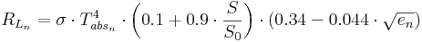
Calculation of the Net Radiation Balance

The energy that is necessary for the evaporation is provided by radiation. The net radiation balance for each day needs to be defined for the calculation of the amount of energy that results from the energy balance segments. The energy fluxes that add to the net radiation balance are: the extraterrestrial radiation, the global radiation, the atmospheric backradiation, the longwave radiation as well as the soil heat flux.

The extraterrestrial radiation (R₀) is calculated against the latitude as well as the annual variation of the insolation angle of the sun (declination):

$R_0= \frac {1}{8.64} \cdot \left[245 \cdot (9.9 + 7.08 \cdot \sin{\zeta})+0.18 \cdot (\phi - 51) \cdot (\sin{\zeta} - 1) \right] \, \, \, \left[\frac{\mathrm{W}}{\mathrm{m^2}} \right]$

with the angle ζ and the factor (1/8.64) for the conversion of Jcm^-2 to Wm^-2, as well as from latitude φ to degree.

The global radiation (R_G) is calculated on the basis of the extraterrestrial radiation R₀ and the cloudiness. The degree of cloudiness is here approximated from the relation of the measured sunshine duration to the astronomic possible sunshine duration for unclouded sky (S₀) with the help of an empirical relation according to the Ångström formula. RG is calculated according to:

$R_G = R_0 \cdot \left( a + b \cdot \frac{S}{S_0} \right) \, \, \, \left[ \frac{\mathrm{W}}{\mathrm{m^2}} \right]$

The calculation of the astronomic possible sunshine duration (S₀) in the annual variation is carried out against the latitude:

$S_0 = 12.3 + \sin{ \zeta} \cdot \left( 4.3 + \frac{\phi -51}{6} \right) \, \, \, \mathrm{[h]}$

with

ζ = 0.0172*JT - 1.39

JT ... Julian day [1...365;366]

φ ... latitude

The longwave radiation of the earth’s surface and the atmospheric backradiation are calculated together as effective longwave radiation (R_L). The black body radiation according to Boltzmann, the degree of cloudiness and an empiric function of the air‘s content of water vapor are part of the calculation:

$R_{L_d} = \sigma \cdot T_{abs_d}^4 \cdot \left( 0.1 + 0.9 \cdot \frac{S}{S_0} \right) \cdot \left( 0.34 - 0.044 \cdot \sqrt{e_d} \right)$

$\left[ \frac{\mathrm{W}}{\mathrm{m^2}} \right]$

$R_{L_n} = \sigma \cdot T_{abs_n}^4 \cdot \left( 0.1 + 0.9 \cdot \frac{S}{S_0} \right) \cdot \left( 0.34 - 0.044 \cdot \sqrt{e_n} \right)$

with

σ ... Stefan-Boltzmann-constant (=5.67*10-8) [Wm^-2K^-4]

T_{abs_d,n} ... absolute air temperature [K]

e_d,n ... vapor pressure of the air [hPa]

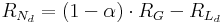
The net radiation results from global radiation (R_G) reduced by the albedo (α) of the particular land use type as well as from the effective longwave radiation (R_L):

$R_{N_d} = (1- \alpha) \cdot R_G - R_{L_d}$

$\left[ \frac{\mathrm{W}}{\mathrm{m^2}} \right]$

$R_{N_n} = 0 - R_{L_n}$

The soil heat flux (G) is then calculated according to the very much simplified relation:

$G_d = 0.2 \cdot R_{N_d}$

$\left[ \frac{\mathrm{W}}{\mathrm{m^2}} \right]$

$G_d = 0.2 \cdot R_{N_n}$

Calculation of Live Stock Specific Parameters

The influence of different vegetation forms on the evaporation is taken into account via two resistances in the Penman-Monteith-approach: the surface resistance (r_s) and the aerodynamic resistance (r_a). For the calculation of the resistances, land use-specific parameters are needed. These are: the leaf area index LAI, the effective vegetation height (eff.Bh.), and the surface resistances for water saturation. Their values are shown for different land cover classes in the following table:

Land use parameters of different land cover classes

Furthermore, the live stock specific albedo values are contained which are used for the calculation of the net radiation balance. The leaf area index and the effective vegetation height are represented as distinctive points (d₁...d₄) of the year. The points represent the beginning of the vegetation period (d₁), the reaching of the maximum development or ripeness (d₂), the ripeness period until the point d₃ and then the decrease until the end of the vegetation period (d₄). The individual points are represented by the Julian days (d₁ = 110, d₂ = 150, d₃ = 250, d₄ = 280) for areas at about 400m height. For other heights (z) these points are approximated according to the following empirical relation:

$d_1(z)=d_1(400)+0.025 \cdot (z-400)$

$d_2(z)=d_2(400)+0.025 \cdot (z-400)$

$d_3(z)=d_3(400)+0.025 \cdot (z-400)$

$d_4(z)=d_4(400)+0.025 \cdot (z-400)$

The values between the individual points are interpolated linearly. The aerodynamic resistance (ra) of the particular land use type can be calculated according to the following equation:

$ra = \frac{4.72 \cdot \left( \ln{ \left( \frac{z_m}{z_0} \right)} \right)^2}{1 + 0.54 \cdot v_2} \, \, \, \left[ \frac{\mathrm{s}}{\mathrm{m}} \right]$

with

z_m ... measuring height of the wind speed (=2 m) [m]

z₀ ... aerodynamic roughness length (≈ 0.125*effective vegetation height) [m]

v₂ ... wind speed at 2 m height [ms^-1]

The aerodynamic resistance for effective vegetation heights of equal or more than 10 m can be calculated according to the following simplified equation:

$ra = \frac{64}{1 + 0.54 \cdot v_2} \, \, \, \left[ \frac{\mathrm{s}}{\mathrm{m}} \right]$

The surface resistance of the particular use type is calculated according to the following equation:

$rs_d = \left( \frac{1-A}{rsc} + \frac{A}{rss} \right)^{-1} \, \, \, \left[ \frac{\mathrm{s}}{\mathrm{m}} \right]$

$rs_n = \left( \frac{LAI}{2500} + \frac{1}{rss} \right)^{-1} \, \, \, \left[ \frac{\mathrm{s}}{\mathrm{m}} \right]$

with

rsc ... surface resistance [sm^-1]

A ... 0.7^LAI [-]

rss ... surface resistance of uncovered soil [sm^-1]

Specific Adaptation of Evaporation during the Modeling

Furthermore, slope and aspect significantly influence the evaporation amount and are therefore taken into account by the following correction factors:

$Korr_{ETP} = (0.01605 \cdot \sin{( \delta -90)} - 0.00025 ) \cdot \alpha + 1$

with

δ ... aspect from north in degree

α ... slope in degree

The evaporation of slopes (ETP') is calculated with the help of this correction factor:

$ETP' = ETP \cdot Korr_{ETP} \, \, \, \mathrm{[mmd^{-1}]}$

For the consideration of the current soil humidity the particular correction functions are applied. It is assumed that the vegetation can only transpire until a particular water content of the soil with the potential evaporation rate is reached. After going below this water content, the real evaporation decreases proportionally to the potential evaporation until it becomes zero at the point of the permanent wilting point. In J2000 there is a linear function with the calibration coefficient linear_reduc and a non linear procedure with the calibration coefficient poly_reduc available for the reduction:

$f(\Theta)= \begin{cases} \left( \frac{\Theta MPS}{linear_-reduc} \right) & \mathrm{f\ddot{u}r} \, \, \, linear_-reduc < \Theta MPS \\ \, \, \, 1 & \mathrm{sonst} \end{cases} \, \, \, [-]$

$f(\Theta) = 10^{\left(-10 \cdot (1-sat)^{poly_-reduc} \right)} \, \, \, [-]$

With the linear function it is assumed that the current ETP conforms to the potential ETP as long as the relative MPS saturation equals or is greater than the linear_reduc. If the relative MPS saturation falls below the linear_reduc, the reduction factor f(Θ) decreases linearly. Thus, linear_reduc represents a threshold that needs to be defined by the user and that can take values from 0 to 1. In contrast, the calibration coefficient poly_reduc can take all values between zero and infinite. For a small value of poly_reduc the reduction factor is also reduced for a high MPS saturation. If the values of poly_reduc increase, the potential ETP slightly decreases. For decreasing MPS saturation, a higher reduction occurs. The real evaporation is calculated with the value from the correction function against the current water content of the soil from the potential evaporation (ETP'):

$ETR = f(\Theta) \cdot ETP' \, \, \, \mathrm{[mm d^{-1}]}$

Interception Module

The interception module serves the calculation of the net precipitations from the field precipitations against the particular vegetation covers and their development in the annual variation. The field precipitation is reduced by the interception part to the net precipitation via interception. Thus, net precipitation only occurs when the maximum interception storage capacity of the vegetation is exhausted. The surplus is then passed on as through falling precipitation to the following module. The maximum interception capacity (Int _max) is calculated in J2000 according to the following formula:

$Int_{max} = \alpha \cdot{LAI} \, \, \, \mathrm{[mm]}$

with

α ... storage capacity per m2 leaf area against the precipitation type [mm]

LAI ... leaf area index of the particular land use class [-]

The parameter α has a different development, depending on the type of the intercepted precipitation (rain or snow), since the maximum interception capacity of snow is noticeably higher than of liquid precipitation. The leaf area index for the individual vegetation types of the year is calculated with the described method for each day of the time series. The emptying of the interception storage is carried out exclusively by evaporation. A special case occurs when the development of the parameter α changes from rain to snow due to the air temperature. This leads to a heavy decrease of the maximum interception storage capacity. Possible surplus is passed on as draining precipitation to the following module.

Snow Module

The snow development is subdivided into three phases in the snow module of J2000: the snow accumulation, the metamorphosis and the snow melt. The amount of snow of the total precipitation is defined via the air temperature in order to calculate the daily accumulation rate (Acc). For this purpose, it is assumed that going below a particular threshold temperature the total precipitation consists of snow and for going above a second threshold temperature the total precipitation consists of rain. In the zone between these threshold temperatures a mixed precipitation occurs. In order to define the threshold temperatures and therefore the size of the transition zone, a temperature value (Trs in °C) needs to be given which conforms to the temperature where 50% of precipitation is snow and 50% is rain. Additionally, a parameter Trans (in K) needs to be defined that is taken as the half width of the transition zone. The real snow proportion (p(s)) of the daily precipitation against the air temperature (T) is calculated according to:

$p(s) = \frac{TRS + Trans - T}{2 \cdot Trans} \, \, \, \mathrm{[mm]}$

The daily amount of snow (N_s) or amount of rain (N_r) is calculated according to:

$N_s = N \cdot p(s) \, \, \, \mathrm{[mm]}$

$N_r = N \cdot (1-p(s)) \, \, \, \mathrm{[mm]}$

The so calculated snow water equivalent is allocated to the solid storage (SWCdry). If p(s) is less than 1.0, the resulting amount of rain is added to the liquid storage.

The resulting snow height change is calculated with the help of the density of fresh snow (ρ_new):

$\Delta SH = \frac{N_s}{\rho_{new}} \, \, \, \mathrm{[mm]}$

The thermal circumstances under the snow cover are taken into account with the store of cold in the snow cover in connection with the snow melt. Since melted water freezes immediately due to negative isothermal circumstances under the snow cover and thus, the runoff is stopped, the store of cold needs to reach the value zero so that the process of snowmelt begins. Consequently, negative temperatures raise the store of cold whereas positive temperatures reduce it. The calculation of the store of cold (CC) results from the product of the air temperature by a calibration parameter (coldContFac):

$CC = coldContFac \cdot T \, \, \, \mathrm{[mm]}$

The snow cover can store liquid water in its pores until a certain critical density (critDens). This storage capability is lost nearly completely and irreversibly when a certain amount of liquid water proportionally to the total snow water equivalent (between 40% and 45%) is reached. This is taken into account in the modeling by the calculation of the maximum water content (WS_max) of the snow cover:

$WS_{max} = critDens \cdot snowDepth \, \, \, \mathrm{[mm]}$

The critical density (critDens) needs to be given by the user. The stored water in the snow cover that goes beyond this threshold is drained:

$SMR = \left( 1- e^{(1-(\frac{critDens}{totDens}))^4} \right) \, \, \, \mathrm{[mm]}$

The resulting snow water (SMR) is used as input value in the following soil module. The snow cover’s density keeps the value of the critical density until the snow cover thaws or goes back into the accumulation phase due to new snowfall.

In J2000 there are two methods available for the calculation of the potential melting rate: a simple method is based on the tight relation of air temperature and the snowmelt intensity. The potential melting rate (potMR) is calculated on the basis of air temperature, the day degree factor (ddf) and the total snow density (totSnowDens):

$potMR = ddf \cdot totSnowDens \cdot T \, \, \, \mathrm{[mm]}$

The day degree factor represents an empirically generated thawing coefficient. Alternatively to the mentioned calculation formula, the potential melting rate can also be calculated via a more complex approach. In addition to the amount of precipitation (P in mm) and the air temperature, further energy fluxes (air temperature, precipitation temperature and soil temperature) are taken into account in this calculation. Since the necessary input data for this approach (e.g. precipitation intensity, heat of fusion, and wind speed) are often unavailable, they need to be calibrated. The so resulting and simplified equation only contains the temperature data, precipitation data and the calibration factors r_factor, g_factor and t_factor that need to be generated empirically.

$potMR = t_-factor \cdot T + r_-factor \cdot P + g_-factor \, \, \, \mathrm{[mm]}$

Soil Water Module

The soil module is structured in process units (infiltration, evapotranspiration) and store units (middle pore storage = MPS, large pore storage = LPS, depression storage). At first, the infiltration capacity against the water saturation in the soil and a maximum infiltration rate is estimated with the help of an empirical method. The maximum infiltration rate functions as threshold. When this threshold is crossed, the surplus water is stored in the depression storage or lead into the direct surface runoff. The maximum amount of water that can be held back in surface depressions is seen as maximum depression storage (maxDepStor). Furthermore, the depression storage is dependent on the surface structure as well as on the slope and is halved when the slope is greater than 5%. The precipitation water that is not infiltrated or stored in the depression storage drains as surface runoff. In order to calculate the infiltration (Inf), an empirical calculation method is used in J2000. For this purpose, a maximum infiltration rate (maxINF in mm/d), defined by the user, against the relative saturation deficit of the soil (1 - soil_sat) is taken into account:

$Inf = (1-soil_{sat}) \cdot maxINF \, \, \, \mathrm{[mm/d]}$

The calculation of the relative saturation of the soil is carried out according to:

$soil_{sat} = \frac{(MPS_{act} + LPS_{act})}{(MPS_{max} + LPS_{max})} \, \, \, [-]$

with

MPS_act, MPS_max ... actual, maximum filling of the middle pore storage

LPS_act, LPS_max ... actual, maximum filling of the large pore storage

Three infiltration scenarios are considered for the definition of the maximum infiltration rate. The setting of the maximum infiltration rate (maxINF), defined by the user, with the parameter Inf_winter is the normal case of the infiltration for the winter half year. Additionally, the special infiltration conditions for the convective precipitation with short duration and high intensity that occur in summer are taken into account via the parameter Inf_summer. Furthermore, with the setting of the parameter Inf_snow, the circumstance of decreased infiltration due to partly or complete frozen soil when snow cover occurs shall be taken into account. If the amount of water that is to be infiltrated is greater than the maximum infiltration rate (maxINF) set up by the user, the surplus water is stored in the depression storage or drains as surface runoff. Furthermore, the infiltration is influenced by the sealed grade of the surface. For a sealed grade greater than 80% (impervious areas IP>80) only 25% of the precipitation infiltrates; for a sealed grade less than 80% (impervious areas IP<80) 60% of the precipitation infiltrates. The infiltrated precipitation is allocated to the middle pore storage and the large pore storage whereby the saturation deficit of the MP is determining. The influx in the MPS (MPS_in) results from the infiltrated precipitation (Inf) against its relative storage content (ΘMPS) as well as from a calibration coefficient (Dist coef) set up by the user. MPSin is calculated according to the following equation:

$MPS_{in} = Inf \cdot \left( 1-e^{(\frac{-1 \cdot Dist coef}{\Theta MPS})} \right) \, \, \, \mathrm{[mm]}$

The infiltrated amount of precipitation water which is not absorbed by the MPS goes into the large pore storage (LPS_in):

$LPS_{in} = Inf - MPS_{in} \, \, \, \mathrm{[mm]}$

The value range of the calibration coefficient lies between zero (so that no water can flow into the MPS) and infinite. The discharge from the MPS is exclusively carried out via evapotranspiration (ETP), which is calculated from the current storage filling of the MPS and the potential ETP (see calculation of evapotranspiration).

The vertical (percolation) and lateral (interflow) water movement in the ground exclusively occurs in the LPS and is therefore dependent on the amount of the large pores. At first, the all in all runoff from the LPS (LPSout) which finally divides into the two mentioned runoff components needs to be calculated. It is calculated against the relative saturation of the soil (soilsat), the actual large storage content (LPSact) and a calibration coefficient (LPSout).

$LPS_{out} = (soil_{sat})^{LPSout} \cdot LPS_{act} \, \, \, \mathrm{[mm]}$

The following allocation of the LPS runoff in the vertical and lateral (inter) flow direction is carried out against the slope and a user specific calibration factor (LatVertDist) which can take values between zero and infinite.

$perc = LPS_{out} \cdot (1- \tan{(Hangneigung)} \cdot LatVertDist) \, \, \, \mathrm{[mm]}$

$inter = LPS_{out} \cdot (\tan{(Hangneigung)} \cdot LatVertDist) \, \, \, \mathrm{[mm]}$

The percolation rate can be restricted by a user specific maximum, absolute, daily percolation rate (maxPerc). When the maximum percolation rate is crossed, the surplus water is led to the interflow. The maximum percolation rate results from the hydraulic permeability and the amount of large pores and macro pores and can be estimated only vaguely. The water that is in the LPS after a time step can diffuse in the MPS (LPS2MPS) when the actual LPS storage content (LPSact), the relative saturation of the MPS (ΘMPS) and the calibration coefficient Diff coef are considered:

$LPS2MPS = LPS_{act} \cdot \left( 1-e^{(\frac{-Diffcoef}{\Theta MPS})} \right) \, \, \, \mathrm{[mm]}$

The calibration parameter Dist coef also possesses a theoretical value range from 0 to infinite. No diffusion takes place for values of 0. When the value 5 is crossed, nearly the entire water that remained in the large pores diffuses in the MPS.

While the percolation is limited by the maximum percolation rate, the discharge can be decelerated via the direct runoff (RD1) and the interflow (RD2) by user-defined retention coefficient (recRD1, recRD2):

$Abfluss = \frac{1}{rec} \cdot Abflusskomponente \, \, \, \mathrm{[mm]}$

If recRD1 or recRD2 gets a greater value than1, the runoff is decelerated and the surplus water remains in the particular storages until the next time steps. Equally, a small value for k leads to an increase of the runoff.

Ground Water Module

The model concept of the ground water module in J2000 offers the viewing of the ground water runoff of all geologic formations that occur in the catchment area in consideration of the different storage and runoff behaviours. In the individual geologic units there is a distinction between the upper ground-water reservoir (RG1) in loose weathered material with high permeability and the lower ground-water reservoir (RG2) in fractures and clefts of the bedrock. Consequently, two basis runoff components are generated: a fast one from the upper ground-water reservoir and a slow one from the lower ground-water reservoir. The filling of the ground-water reservoir results from the vertical runoff component of the soil module. The emptying can be carried out by the lateral subterranean runoff components as well as capillary elevation in the unsaturated zone. The parameterization of ground-water reservoirs is carried out with the definition of the maximum storage capacity of the upper (maxRG2) and the lower (max RG1) ground water reservoir as well as a retention coefficient each for both reservoirs (recRG1) and (recRG2). Both parameters need to be determined for each geologic entity separately. The maximum storage capacity results from the product of the cavity and the thickness of the individual storage per m² unit area. The calculation of the water yield is carried out against the actual storage fillings as a linear drain function. The storage retention coefficients, which are to be seen as residence times of the water in the storage of interest, are taken into account as factor of the actual storage content (actRG1 and actRG2) for the calculation of the ground water runoff (outRG1 and outRG2):

$out RG1 = \frac{1}{gwRG1Fact \cdot{recRG1}} \cdot{actRG1} \, \, \, \mathrm{[mm]}$

$out RG2 = \frac{1}{gwRG2Fact \cdot{recRG2}} \cdot{actRG2} \, \, \, \mathrm{[mm]}$

In order to take the ground water reservoirs’ runoff dynamics in the catchment area into account, the ground water runoffs outRG1 and outRG2 can be multiplied by the calibration parameters gwRG1Fact or gwRG2Fact for the particular upper or lower ground water reservoir. The given parameter settings of these factors take the value one, whereby the value must not be less than zero. Generally, the runoff from the ground-water reservoirs is carried out faster when a small factor is given and slower when a big factor is given.

For a further adaptation to the catchment area, the calibration coefficient gwRG1RG2dist has to be set up. It influences the allocation of the percolation water from the soil module (perc) to both ground water reservoirs for each Hydrological Response Unit in consideration of the slope. The calibration parameter disttRG1RG2 is used as exponent in the calculation of the ground water influx (inRG1 and inRG2):

$inRG1 = perc \cdot{(1 - ( 1 - \tan{(Hangneigung)))}} \cdot{gwRG1RG2dist} \, \, \, \mathrm{[mm]}$

$inRG2 = perc \cdot{(1- \tan{(Hangneigung)})} \cdot{gwRG1RG2dist} \, \, \, \mathrm{[mm]}$

In addition to the mentioned parameters, the capillary elevation of the ground water (GW2MPS) has an important influence on the soil storage filling in plane areas with very high ground water level, e.g. in wide flood lands. In order to take that circumstance into account, the still free middle pore storage (deltaMPS), which results from the difference of the maximum middle pore storage and the actual middle pore storage volume, is multiplied by an empirically generated factor. The calibration coefficient gwCapRise as well as the relative saturation of the MPS (ThetaMPS) are used for the calculation of this factor:

$GW2MPS = \Delta MPS \cdot{ \left(1 - e^{\frac{-gwCapRise}{ \theta MPS}} \right)} \, \, \, \mathrm{[mm]}$

The calibration coefficient gwCapRise can take values from zero to infinite. However, the capillary elevation is forbidden when the coefficient takes the value zero.

Lateral Routing

The lateral routing module describes the water transfer within a flow cascade from HRU to HRU from the upper catchment area until the receiving stream. Since the retention mechanisms of the runoff are described by the other process modules, here only the HRU‘s influxes and discharges are allocated. The water transfer between the HRUs are seen as n:1 relation. Thus, an HRU can have several influxes but only one discharge. The order of the HRUs as receivers is determined by the topologic ID of the HRU dataset. In the HRU dataset it is also determined which HRUs finally drain in the receiving stream.

Reach Routing

The Reach Routing module describes the flow phenomena in the channel via a cinematic wave-like normal mode and the calculation of the rapidity of flow according to MANNING & STRICKLER. The only parameter (TA) that needs to be set is a routing coefficient which must be set by the user. It represents the travel time of the discharge wave which moves from the channel to the runoff after a precipitation event. Its value as well as the stream’s rapidity of flow (v) and the flow length (fl) are needed for the calculation of a runoff retention coefficient (Rk).

$Rk = \frac{v}{fl} \cdot TA \cdot 3600 \, \, \, [-]$

At first, the rapidity of flow (v_new) with the roughness factor by Manning (M), the slope of the river bed (I) and the hydraulic radius (Rh) need to be set, however. The hydraulic radius (Rh) in turn is calculated from the cross section of the river part where the water flows through (A), from the flow passage (q), the rapidity of flow (v) and the river width (b). For this approach, an initial rapidity of flow (v_init) of 1 m/s is assumed, which is then iteratively abgeglichen with the new calculated rapidity of flow (v_new) until the deviation of both speeds are less than 0,001 m/s.

$Rh = \frac{A}{b+2 \frac{A}{b}} \, \, [m]$ mit: $A = \frac{q}{v_{init}} \, \, \mathrm{[m^2]}$

$V_{new} = M \cdot Rh^{\frac{2}{3}} \cdot I^{\frac{1}{3}} \, \, \mathrm{[m^3/s]}$

Finally, the discharge of the particular river part (q_act) is calculated with the generated runoff retention coefficient (Rk).

$Ausfluss = q_{act} \cdot e^{(\frac{-1}{Rk})} \, \, \mathrm{[m^3/s]}$

The higher the assumed value of TA, the faster the discharge wave moves within a particular period and the less water remains in the channel. The theoretical value range therefore corresponds to the one of positive numbers.

Hydrological Model J2000

Contents

GUI

Input files

Data

Parameters

Regionalization of Climate and Precipitation Data

General Processing

Specific Correction Method and Calculation Method for the Individual Datasets

Calculation of Evapotranspiration

Interception Module

Snow Module

Soil Water Module

Ground Water Module

Lateral Routing

Reach Routing

Views

Personal tools

Navigation

Search

Toolbox

In other languages