Regionalization

From ILMS-Wiki

Regionalization of Climate and Precipitation Data

General Processing

1. Calculation of the linear regression between the daily station values and the elevation of the stations. . Thereby, the coefficient of determination (r²) and the slope of the regression line (b_H) of this relation is calculated. It is assumed that the value (MW) depends linearly on the terrain elevation (H); according to:

$MW = a_H + b_H \cdot H$

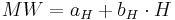
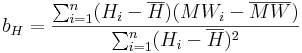
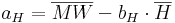
The unknown a_H and b_H are defined according to the Gaussian method of the smallest squares:

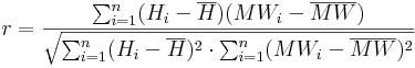
$b_H = \frac{\sum_{i=1}^{n} (H_i - \overline{H})(MW_i - \overline{MW})}{\sum_{i=1}^{n} (H_i - \overline{H})^2}$

$a_H = \overline{MW} - b_H \cdot \overline{H}$

The correlation coefficient of the regression is calculated according to the following equation:

$r = \frac{\sum_{i=1}^{n} (H_i - \overline{H})(MW_i - \overline{MW})}{\sqrt{\sum_{i=1}^{n} (H_i - \overline{H})^2 \cdot \sum_{i=1}^n (MW_i - \overline{MW})^2}}$

2. Definition of the n gaging stations which are nearest to the particular HRU.. The number n which needs to be entered during the parameterization is dependent on the density of the station network as well as on the position of the individual stations.

For each dataset the number of stations (n) that shall be considered for the regionalization needs to be determined in advance. Furthermore, a weighting factor (pIDW) needs to be given. The n-nearest stations are defined according to the following calculation rule with the help of the eastings and northings of all stations as well as the coordinates of the particular HRU. The first step is to calculate the distance (Dist(i)) of each station to the area of interest:

$Dist(i) = \sqrt{(RW_{stat(i)} - RW_{DF})^2 + (HW_{stat(i)} - HW_{DF})^2}$

with

RW ... easting of the station i...n, or the HRU (DF)

HW ... northing of the station i...n, or the HRU (DF)

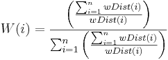
The n stations with the smallest distance to the particular HRU are taken from the distances calculated according to the description above and are then used for further calculations. The distances of these stations are converted to weighted distances (wDist(i)) via potentialization with the weighting factor pIDW. With the help of this weighting factor the influence of nearby stations can be increased and the influence of more distanced stations can be decreased. Good results can be achieved with values of 2 or 3 for the pIDW.

3. Via an Inverse-Distance-Weighted (IDW) the weightings of the n stations are defined dependently on their distances for each HRU. Via the IDW-method the horizontal variability of the station data is taken into account according to its spatial position. The calculation is carried out according to the following equation:

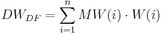
$W(i) = \frac{\left( \frac{\sum\nolimits^n_{i=1} wDist(i)}{wDist(i)} \right)}{\sum^n_{i=1}\left( \frac{\sum\nolimits^n_{i=1} wDist(i)}{wDist(i)} \right)}$

4. The calculation of the data value for each HRU with the weightings from point 3 and an optional elevation correction for the consideration of the vertical variability. The elevation correction is only carried out when the coefficient of determination (calculated under point 1) goes beyond the threshold entered by the user. The calculation without the optional elevation correction is carried out according to the following equation:

$DW_{DF} = \sum^n_{i=1} MW(i) \cdot W(i)$

For data values that possess an elevation effect, an elevation correction for the measured values is carried out additionally when the values have a tight regression relation (r² greater than the threshold entered by the user). The following equation is applied for the calculation:

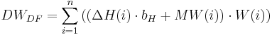
$DW_{DF} = \sum^n_{i=1} \left( ( \Delta H(i) \cdot b_H + MW(i)) \cdot W(i) \right)$

with ΔH(i) ... elevation difference between station i and the HRU

b_H ... slope of the regression line

Specific Correction Method and Calculation Method for the Individual Datasets

Precipitation

Correction of the Moistening Error and Evaporation Error

The correction of the moistening error and evaporation error is carried out according to researches with the help of Hellmann-rainfall gauges by RICHTER (1995). In order to offer a constant correction of the error (which results from the moistening and evaporation loss), logarithmic functions were approximated separately for the summer half year (May-October) and winter half year (November-April) to the discrete tabulated values in the modeling system 2000. If the precipitation height goes beyond the value of 9 mm the moistening error and evaporation error is set to a constant value.

The moistening error and evaporation error for precipitation heights ≤9.0 mm is calculated according to the following equates:

$BV_{Som}= 0.08 \cdot \ln{N} + 0.225 \; \; \; \mathrm{[mm]}$

$BV_{Win}= 0.05 \cdot \ln{N} + 0.13 \; \; \; \mathrm{[mm]}$

For precipitation heights >9.0 mm the moistening and evaporation error is:

$BV_{Som} = 0.47 \; \; \; \mathrm{[mm]}$

$BV_{Win} = 0.30 \; \; \; \mathrm{[mm]}$

Correction of the Wind Error

The quantification of the precipitation error that is to be expected is carried out according to the researches by RICHTER (1995) as function of the precipitation height and the position of the station. It is assumed that the relative wind error (KR_Wind) for rainfall as well as snowfall verhält sich inversely proportional to the precipitation heights (Pm). The calculation is carried out according to the following equations:

$KR_{Wind}= \begin{cases} 0.1349 \cdot P_m^{-0.494} & \mathrm{f\ddot{u}r} \; \; T_{mean} > T_{crit} \\ 0.5319 \cdot P_m^{-0.197} & \mathrm{f\ddot{u}r} \; \; T_{mean} \le T_{crit} \end{cases} \; \; \mathrm{[-]}$

The calculation of the precipitation heights corrected for evaporation error and wind error is then carried out according to the following equation:

$P_{korr} = P_m + P_m \cdot KR_{Wind} + BV_{Som}, BV_{Win} \, \, \, \mathrm{[mmd^{-1}]}$

Temperature

The modeling system J2000 requires values of the day minimum temperature as well as the day maximum temperature. From these values the mean day temperature (T_mean) is calculated as mean average.

The regionalization of the punctual values T_min,T_max and T_mean is carried out according to the rule described above with optional elevation correction.

Wind Speed

The wind speed is not given as direct value from the DWD but as wind force observations (WS) in Beaufort. The conversion of the wind force into the wind speed at 2 m height (v₂) [in ms^-1] can be carried out according to the following equation:

$v_2 = 0.6 \cdot WS^{1.5} + 0.1 \; \; \; \mathrm{[ms^{-1}]}$

This conversion needs to be carried out externally, because J2000 expects the wind speed in m/s.

The conversion of the wind speed at 2 m height to other heights – as it is partly required during the evaporation calculation and the wind correction of the precipitation – is carried out during the modeling according to the following equation:

$v_z = \frac{v_z}{\left( \frac{4.2}{\ln z + 3.5}\right)} \; \; \; \mathrm{[ms^{-1}]}$

The interpolation of the punctual values to the area is carried out according to the method described above. The modeling system allows the inclusion of the optional elevation correction for the regionalization of the wind speed. However, this option should be handled with care, since the wind speed is very dependent on the station’s position.

Sunshine Duration

The daily sunshine duration (S) [in h], is provided as value by the DWD. The interpolation of the station values to the area is carried out according to the procedure described above – without additional calculations or elevation corrections.

Relative Humidity

The relative humidity (U) [in %] can be taken from the DWD as daily values. A direct regionalization of the values is not recommended since they depend on two parameters: the absolute moisture content and the maximum possible moisture content of the air for a particular temperature. Thus, in the J2000 modeling system’s regionalization module the absolute humidity (a) [in g cm^-3] is calculated from the relative humidity and the temperature at the station. It is then regionalized and afterwards the absolute humidity is converted to the relative humidity, again. For this purpose, several calculation steps are necessary which are shown below.

Calculation of the Saturation Vapor Pressure

The saturation vapor pressure (e_s(T)) [in hPa] is calculated according to the Magnus formula with the coefficients by SONNTAG (1994) for the air temperature (T) [in °C]:

$e_s(T) = 6.11 \cdot e^{\left( \frac{17.62 \cdot T}{243.12 + T} \right)} \; \; \; \mathrm{[hPa]}$

Calculation of the Maximum Humidity

The maximum humidity (A) is calculated against the saturation vapor pressure (e_s(T)) and the air temperature (T) according to:

$A(T) = e_s(T) \cdot \frac{216.7}{T + 273.15} \; \; \; \mathrm{[g cm^{-3}]}$

Calculation of the Absolute Humidity

The real water content of the air, the absolute humidity (a) [in gcm^-3], results from the maximum humidity (A)[in gcm^-3] and the relative humidity (U) [in %]:

$a = A \cdot \frac{U}{100} \; \; \; \mathrm{[g cm^{-3}]}$

The so calculated station values of the absolute humidity are then regionalized according to the procedure described above and are converted into relative humidity afterwards. The advantage of this rather complex regionalization method is that, in addition to its higher physical relation, the absolute humidity is more dependent on heights than the relative humidity. Thus, the elevation effect can be used for the regionalization according to the procedure described above. After the regionalization of the absolute humidity, the conversion into relative humidity can be carried out. Instead of the station temperature, the mean air temperature T_mean Anstelle der Temperatur der Station wird aber die zuvor regionalisierte mittlere Lufttemperatur der entsprechenden diskreten Teilfläche gesetzt.

Regionalization