JAMSSCS
Contents |
JAMSSCS
JAMSSCS is a program for the calculation of design discharges for small homogeneous catchment areas. For this purpose, JAMSSCS implements the unit-hydrograph method of the U.S. Soil Conservation Service (SCS) together with the Curve Number (CN) method for the effective rainfall. The program enables the estimation of the runoff in consideration of an approach of a specific design depth of precipitation for small homogeneous catchment areas. The calculations are carried out as far as possible according to the German DVWK rules 112/1982 and 113/1984 and have been adjusted and changed at some points.
JAMSSCS uses the Jena Adapatable Modelling System (JAMS) and is completely written in JAVA. Therefore, it is usable independently from the operating system on different computer configurations.
Note: The decimal separator is the . (period) and not the , (comma) for the data input.
Installation and Quick Start

To tart JAMSSCS, double click on "JAMSSCS.exe". Hereupon, the main window of JAMSSCS appears (JAMS-launcher). The main window contains three tabulators (main group, Kostra-precipitation, individual event), which offer different functions. For the execution of the test dataset only the working directory needs to be set up. The complete path to the JAMSSCS installation directory has to be given here.
With the button [RUN] the model is started.
A new window with three tabulators appears. The first one [JAMSProgress] represents general information on the current model run as text. Should an error or problem arise while executing, an error message might appear in this view. The second tabulator [design discharge] shows the hydrograph of the design discharge in m³/s. The third tabulator [design volume] shows the cumulated volume in million m³. You can zoom into the graphics by left mouse click and pushing of the window. By right mouse click into the graphic a menu opens which allows a certain adjustment, e.g. changing the diagram title, labeling of the axes, background color, frame color, etc. Furthermore, the diagram can be saved as PNG graphic via this menu. The hydrograph can be switched on or off with the help of the checkbox on the right side.
JAMSSCS Input Data
Information that is provided for JAMSSCS always follows a strict format. For tables it is defined as follows:
- Rows that are introduced by # are comment rows which are not processed by the program. Comment rows are only allowed at the beginning of the table. There is no limitation of their number.
- The tabulator is always the column separator
- The order of the columns must always follow the order in the sample tables.
- The first row which is not introduced by # has to contain the row labeling. This labeling should always correspond to the labeling of the tables x and y. The program differentiates between upper and lower case.
- The following rows contain the actual information (separated by the tabulator).
JAMSSCS needs information about the research area and at least the design depth of precipitation. Additionally, a KOSTRA-precipitation file can be read in which contains precipitation heights for different durations and return periods. This file can be read out in XML-format from the KOSTRA-DWD software and can then be processed directly in JAMSSCS.
The necessary area information consists of a description of the hydrological homogeneous areas (HRUs – Hydrological Response Units) that exist in the area given in tables (HRU-table). The output criterion for the generation is the land use and soil type. The calculation of the desired CN-value is carried out on the basis of the reference table (CN table). In the installation there are examples given for both tables which can be adjusted, changed or added. Newly generated input tables for the area description can be given in the main window.
CN Table
The JAMSSCS CN table contains "Curve-Numbers" for different land use-soil-combinations and can be found in the installation directory as “cnNumbers.par”. The Curve-Number describes the part of precipitation that is runoff-effective. It can be interpreted as relative part. The actual calculation of the effective rainfall is described further down with the help of the curve-number.
Table 1: Die CN table of JAMSSCS
| #CN-Numbers | |||||
| LID | soil use | A | B | C | D |
| 1 | settlement (neatly built) | 80 | 80 | 80 | 80 |
| 2 | settlement (loosely built) | 38 | 73 | 89 | 98 |
| 3 | farmland | 64 | 76 | 84 | 88 |
| 5 | deciduous forest | 36 | 60 | 73 | 79 |
| 6 | coniferous forest | 25 | 55 | 70 | 77 |
| 7 | bush, scattered fruit | 45 | 66 | 77 | 83 |
| 9 | grassland | 30 | 58 | 71 | 78 |
| 10 | open areas | 80 | 80 | 80 | 80 |
| 11 | water areas | 100 | 100 | 100 | 100 |
After the comment in the first row, the table contains the column labeling which do not need to be formulated exactly as it is shown here but can also be labeled differently. Note: The order of the columns must be kept in this order. The columns contain:
- LID: A numeric key number for a land cover or land use type, e.g. 3 for farmland (column 1).
- Soil use: A description of the referring land cover or land use type in text form (column 2).
- A, B, C, D: SCS soil types that are described further down (columns 3, 4, 5, and 6).
Then, the entries for the single land cover categories in LID form, description, Curve Number for soil type A, B, C and D follow in the rows. The table can be expanded user-defined via entering new datasets if required. At this, the soil types are defined as follows:
- A: Soils with high infiltration capacity also after heavy pre-moistening, e.g. deep sand or gravel soils.
- B: Soils with middle infiltration capacity. Deep to moderate deep soils with moderate fine or rough texture, e.g. middle deep sand soils, loess, sandy clay.
- C: Soils with low infiltration capacity. Soils with fine to moderate fine texture or water damming layer, e.g. flat sand soils, sandy clay.
- D: Soils with very low infiltration capacity. Clay soils, very flat soils above nearly impermeable material, soils with always high groundwater level.
HRU table
The HRU table contains information about the research area and is structured as follows: (see table 2)
Table 2: HRU table with area information
| #hrus.par | |||
| "ID" | "AREA" | "LID" | "SID" |
| 1 | 0.011 | 3 | B |
| 2 | 1.39 | 4 | B |
| 3 | 0.156 | 7 | B |
| 4 | 0.014 | 8 | B |
| 5 | 0.3 | 11 | B |
The first row without introducing comment symbol (#) contains the labeling for the intern given variables.
The JAMSSCS-component, which this table reads, was generated in a way so exported GIS tables can be read in without further processing. For this reason the labeling must be given exactly as shown above. The permissible labeling are ID, SID, LID, AREA. The names do not need to be given in inverted commas. The order as well as upper and lower case are not important in this table. In addition to the tabulator, the comma (,) can be used as column separator, here.
The first column contains a clear numeric identification number for each hydrological unit; the second column contains the area (in m²), the third one contains the ID (LID) of the dominant land use of the table according to table 1. The fourth column contains the dominant soil type (A-D) – also according to table 1. For the processing of other areas the HRU table always needs to be generated. This can be carried out directly from a GIS. (Tools for automatized derivation in ArcView are described below.)
Further Input Data


The other necessary input data is given directly in the JAMSSCS main window (Figure 1). It is:
- Receiving stream length: The maximum length of the main receiving stream from the source to the runoff in kilometers.
- Deepest, highest point: The topographic height in meters of the deepest point (runoff) and of the highest point (source) of the main receiving stream.
- N-allocation form: Determines the temporal allocation of precipitation. Valid information is: B = block rainfall, rainfall M = in the middle of the event, A = at the beginning of the event and E = at the end of the event .
- Model runtime: Calculation time for the modeling in hours.
- Time step length: Length of a specific calculation time step in seconds.
For the precipitation allocation form the referring temporal allocations are implemented in JAMSSCS and follow the DVWK 113/1984 as far as possible.
Calculation of Individual Events
Individual precipitation events can be simulated with the help of the tabulator individual events. The necessary parameters can be adjusted here. These are:
- Precipitation duration: the temporal duration of precipitation in minutes
- Design depth of precipitation: the amount of fallen precipitation in open land which is reduced to effective rainfall in the model run
- Individual-Q-output: file name for an output file that is to be generated in which the calculated values can be saved. It is a simple ASCII-file which can be further processed with text editors as well as table calculations. The file name has to be given in consideration to the working directory. The file contains the runoff in m³/s for each time step as well as the temporally cumulated runoff volume in million m³.
- Decimal places: the number of decimal places for the values in the output file.
- Runoff-plot: the graphic output of hydrographs can be switched on or off here
The following fields serve the configuration of the model output. These are:
- Legend: labeling of the legend which is additionally complemented automatically by the precipitation height
- Line color: labeling for the color of the hydrograph. Valid labeling are for example "blue", "red", "green", "black" etc.
- X,Y-axes labeling: axes labeling (can also be changed later)
- Volume-plot: generates a graphic presentation of the temporally cumulated runoff volume in million m³.
Calculation with KOSTRA-Precipitation


The product KOSTRA-DWD contains the storm rainfall heights for Germany in dependence of the duration and return period in the area of the durations D between 5 minutes and 72 hours as well as in the area of the yearly return periods between T = 0.5 a (according to the yearly exceedence frequency of n = 2x per year in the mean) and T = 100 a (in the mean all 100 years only once received or exceeded according to n = 0.01).
KOSTRA-DWD allows the export as XML-file which can be read directly from JAMSSCS. Such a file contains all values of a KOSTRA-DWD grid cell.
The calculations are carried out with the precipitation allocation form given in the tabulator main group. Further necessary settings are provided in the tabulator KOSTRA precipitation in JAMSSCS. These are:
- Kostra on: Switches KOSTRA calculations on or off
- Kostra-runoff-plot: Switches the graphic output of the hydrograph for KOSTRA calculations on or off
- Kostra-volume-plot: Switches the graphic output of the cumulated volume for KOSTRA calculations on or off
- Kostra-input-file: the exported XML-file from KOSTRA-DWD. The complete path name has to be given here, e.g. E:\Projekte\JAMSscnMethod\KOSTRA-DWD-Tabelle-S48-Z56 Jena.xml.
- Return period: either one of the valid KOSTRA return periods (0.5, 1, 2, 5, 10, 20, 50, 100) or each other return period which must be bigger than 100 years, though. The referring precipitations are calculated according to the PEN-method in this case. If a return period of more than 100 years is chosen in the field, the checkbox “PEN-precipitation on:” must be selected.
- Kostra-detail: a file name for the detail text output of a KOSTRA simulation. The file name is completed intern via the working directory. This file contains runoff data for each time step and for each combination of a KOSTRA simulation. The output format is a text file separated by tabulator.
- Kostra-summary: a compressed form of the results of a KOSTRA simulation which contains the maximum peak discharge and the volume of each calculated KOSTRA simulation
- Decimal places: the number of decimal places for the values in the output file
- Variable precipitation return period: If the checkbox is activated, the calculation with the precipitation duration, given in the tabulator individual event, and all return periods shown above is carried out. The valid precipitation durations are: 5, 10, 15, 20, 30, 45, 60, 90, 120, 180, 240, 360, 540, 720, 1080, 1440, 2880, 4320 minutes.
- Variable precipitation duration: If the checkbox is activated (and the one above is deactivated), the calculation for the return period given above and all precipitation durations given above is carried out.
- PEN-precipitation on: with the help of this checkbox the calculation of precipitation with very high return periods, which go beyond the 100 years return interval of the KOSTRA-values, is switched on or off. (The calculation of the PEN-precipitations is described further down.)
- PEN return periods: a list of return periods for which the PEN-calculation shall be carried out. The values of the list have to be separated by semicolon (;).
Intern Calculations - SCS Theory, PEN-Precipitations
The intern calculation of the unit hydrograph is based on the calculation of the effective rainfall in dependence of the CN-value of the catchment area and linear reservoirs in series (Nash-cascade) with two storages with different discharge coefficients (k1,2) as well as the variable allocation of the precipitation to the two storages. The first storage represents the fast direct runoff; the second represents the decelerated basis runoff.
CN-Value Calculation
An area-weighted mean CN-value, based on the entries of the HRU table and the CN table, is calculated for the area. The calculation is carried out according to the following equation:
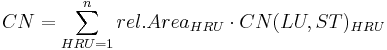
rel.Area is the relative area part of the HRU and CN(LU, ST) is the entry referring to the HRU in the CN table.
The Effective Rainfall
The effective rainfall (hNe) describes the runoff-effective amount of the total precipitation. The calculation is carried out according to the following exponential function:
![h_{Ne} = \frac{\left[ (h_N / 25.4) - (200/CN) + 2 \right]^2}{(h_N / 25.4) + (800 / CN) - 8} \cdot 25.4](/ilmswiki/uploads/math/8/2/d/82d7134d815cb6e36678c73f7a44d724.png)
hN is the design depth of precipitation (in mm) and CN is the CN-value according to equation 1. The minimal level for the design depth of precipitation (UGN) where an effective rainfall > 0 occurs results when hNe is set to zero:
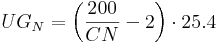
For a design depth of precipitation less than or equal to the minimal level (UGN) an effective rainfall of 0 mm results, thus.
Allocation of the Effective Rainfall
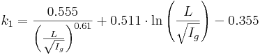
The effective rainfall which is calculated according to the presented equations above is allocated to the two storages of the storage cascade based on the calculation of the coefficients β1,2. β1 is calculated on the basis of receiving stream length (L) and the receiving stream difference (Ig = (HP – TP) / L) according to:
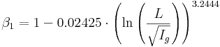 for
for 
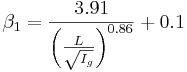 for
for 
The coefficient β2 results from 1 – β1. Due to this allocation the first storage (direct runoff part) of the cascade gets relatively more precipitation in steep areas and less in flat areas.
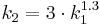
Linear Reservoirs in Series
The calculation of the unit hydrograph is carried out via linear reservoirs in series with two storages that have different retention coefficients (k1,2). These are calculated according to:
For each of the two storages a unit hydrograph based on the k-values is then calculated according to the following equation:
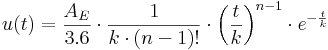
with:
| t | time step in seconds |
| AE | size of the catchment area in km² |
| n | number of storages(in this case: always 2) |
| k | the retention coefficient according to the equations given above |
The total runoff of the area results from the sum of both runoff components, then.
Practice-Oriented Extreme Values of the Precipitation (PEN)
The estimation of precipitation with return periods or return intervals which are less frequent than the 100 years of the KOSTRA-data is carried out according to the modified PEN-method (Gewässerkundlicher Landesdienst Thüringen: Anforderungen an Hydrologische Gutachten, Fassung vom 31. Mai 2005). With this method precipitations for arbitrary rare return intervals based on the KOSTRA-data for each KOSTRA-duration are extrapolated.
The calculations for a precipitation P with a return interval T and an arbitrary duration is carried out according to:
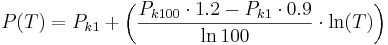 ,
,
Pk1 of the KOSTRA-precipitation with return interval is 1 year and Pk100 of the KOSTRA-precipitation with return interval is 100 years of the referring duration.
HRU Parameter Definition in ArcView
The parameter table can be generated with the GIS ArcView quite simply. The necessary data and steps are described in the following part.
Necessary Data Areas
For the processing the following data areas must be available:
- Soil map with CN-coding (A-D) – available for the entire land Thuringia (The input map has to contain a field with the name “SID” in which the CN-coding (A-D) is saved!)
- Land use with referring coding – available for the entire land Thuringia (The input map has to contain a field with the name “LID” in which the clear numeric coding for the land use units is saved!)
- Shape file of the catchment area
- Shape file of the main receiving stream (optional)
- digital terrain model (optional)
All data areas must be available in a consistent reference system (e.g. Gauss-Krüger).
Conditions in ArcView

- Geoprocessing
- Spatial Analyst (only required when elevation model is used)
- JAMSSCS extension (jamsscs.avx)
The extension jamsscs.avx (downloadable under the link above) must be copied into ArcView’s extension directory (EXT32). This can generally be found under: C:\ESRI\AV_GIS30\ARCVIEW\EXT32.
The installation of the JAMSSCS extension adds a new menu (JAMSSCS) in ArcView which is visible when a View is active. This menu contains three entries that are described in more detail further down. Whether the extensions are installed and activated can be checked under the menu item file --> check extensions.
Clipping of Input Data

- Start "GeoProcessingWizard" in the menu JAMSSCS --> GeoProcessing...
- Select the subitem "Clip" in the appearing dialogue and confirm with the button [Next]
- Select the soil map or land use map in the upper ListBox ("select input theme that shall be clipped:") and the catchment area border in the second ListBox ("select Polygon overlay theme:"). For both the checkbox "only use selected objects" must be deselected.
- Optionally, an output file name can be given in the third ListBox ("give output file").
- The process is started with the button [Finish].
When the steps described above are carried out for both input maps, cut versions of the land use and soil map are available for further processing, then.
Overlaying Input Data

- Select "Intersect themes" then click [Next]
- Select the cut land use in the first ListBox
- Select the cut CN-coded soil map in the second ListBox
- Optionally, a file name for the output file (e.g. "hrus.shp") can be given.

Refreshing the Attribute Table
For the use in JAMSSCS the attribute table of the generated HRU-theme must be refreshed and extended. This is carried out as follows:
- Adding a clear numeric ID for each polygon
- Deleting surplus attributes
- Calculation and adding of the area in m² for each polygon
For this purpose, the HRU-theme has to be selected in the view at first. Then, the attribute table is extended with the necessary information via the menu item "JAMSSCS --> refresh table...".
Exporting the Attribute Table
The extended attribute table must be exported finally in order to be processed with JAMMSCS at a later point. For this purpose, the HRU-theme in the view must be active. The export is then carried out with the menu item "JAMSSCS-->export table...". The program asks for a file name and starts the export, then.
Bibliography
DVWK-Regeln zur Wasserwirtschaft, H. 112/1982: Arbeitsanleitung zur Anwendung von Niederschlags-Abfluss-Modellen in kleinen Einzugsgebieten; verantw. Herausg. Dt. Verb. für Wasserwirtschaft u. Kulturbau e.V. (DVWK). Bearb. vom DVWK-Fachausschuss "Niederschlag-Abfluss-Modelle" - Hamburg, Berlin: Parey; Teil I: Analyse; DK 556.161.072 Niederschlag-Abfluss-Modelle, DK 556.51.028 Kleineinzugsgebiete. - 1982.
DVWK-Regeln zur Wasserwirtschaft, H. 113/1984: Arbeitsanleitung zur Anwendung von Niederschlags-Abfluss-Modellen in kleinen Einzugsgebieten; verantw. Herausg. Dt. Verb. für Wasserwirtschaft u. Kulturbau e.V. (DVWK). Bearb. vom DVWK-Fachausschuss "Niederschlag-Abfluss-Modelle" - Hamburg, Berlin: Parey; Teil 2: Synthese; DK 556.161.072 Niederschlag-Abfluss-Modelle, DK 556.51.028 Kleineinzugsgebiete. - 1984.
Editing and Contact
| Dr. Peter Krause | Dr. Claudia Liese |
| Lehrstuhl Geoinformatik | Referat 51 - Gewässerökologie, Hydrologie, Wasserbau |
| Institut für Geographie | Abteilung 5 - Wasser, Boden, Altlasten, Wismut |
| Friedrich-Schiller-Universität Jena | Thüringer Landesanstalt für Umwelt und Geologie |
| Tel. 03641-948864 | Tel. 03641-684518 |
| email: p.krause@uni-jena.de | email: c.liese@tlugjena.thueringen.de |